Gini and Entropy in Decision trees
Introduction
Decision trees is a popular method along with linear regression, but how does it work? If you look at sklearn’s decision tree classifer:
1
2
3
4
5
6
7
8
9
10
11
12

class sklearn.tree.DecisionTreeClassifier(*,
    criterion='gini',
    splitter='best',
    max_depth=None,
    min_samples_split=2, min_samples_leaf=1,
    min_weight_fraction_leaf=0.0,
    max_features=None,
    random_state=None,
    max_leaf_nodes=None,
    min_impurity_decrease=0.0,
    class_weight=None,
    ccp_alpha=0.0)
There is criterion=gini. If you go further down the docs, it says: criterion{“gini”, “entropy”}, default=”gini” which is further defined by function to measure the quality of a split. Supported criteria are “gini” for the Gini impurity and “entropy” for the information gain.
So, what exactly is
- entropy? gini?
- How does it help you to find which feature to split?
- What about continuous variables? How does it find with values to split?
- What if you have a continuous target then?
Entropy
Entropy is defined as:
\[H(X) = -\sum_i^N P(x_i) \log P(x_i)\]Interesting fact why H is being used to define entropy
Note, this is different from cross entropy which is defined as:
\[H(p,q) = -E_p[log_q] = \sum_i^N P(x_i)\log(Q(x_i))\]For example the cross entropy in logistic regression is defined as:
\[-\frac{1}{N}\sum_i^n \bigg[y_i\log(\hat{y}_i) + (1-y_i)\log(1-\hat{y}_i)\bigg]\]
Now, let’s create a fake dataset, fruits with apples, banana and pear. Your task is to run a decision classifier to predict which fruit it is based on it’s attributes.
1
2
3
4
5
6
7
8
9
10
11
12
13
14
15
16
17
18
19
20
21
22
23
24
25
26
27
28
29
30
31
32
33
34
35
36
37
38
39
40
41
42
43
44
45
46

from typing import List, Tuple, Callable
from math import log
from scipy.stats import entropy
import numpy as np
import pandas as pd

N, N_TYPES = 1000, 3
PROPORTION: List[float] = [0.5, 0.3, 0.2]
FRUITS: List[str] = ["apple", "banana", "pear"]
COLORS: List[str] = ["red", "yellow", "green"]
SIZE: List[str] = ["small", "big"]
np.random.seed(0)


def assign_colors(input_fruit: str) -> str:
    if input_fruit == "apple":
        # Apple can be red and green
        # but majority of apples are considered red
        return np.random.choice(COLORS, size=1, p=[0.9, 0.01, 0.09])[0]
    elif input_fruit == "banana":
        # Banana can be green in color until it is ripe
        # but widely accepted that it is yellow
        return np.random.choice(COLORS, size=1, p=[0.01, 0.75, 0.24])[0]
    else:
        # Some pear can be red, yellow, or green - but mostly green
        return np.random.choice(COLORS, size=1, p=[0.05, 0.35, 0.6])[0]


df = pd.DataFrame(
    dict(
        target=np.random.choice(FRUITS, size=N, replace=True, p=PROPORTION),
        size=np.random.choice(SIZE, size=N, replace=True, p=[0.5, 0.5]),
    )
).assign(color=lambda df: df.apply(lambda col: assign_colors(col["target"]), axis=1))

df.sample(5)

"""
	target	size	color
144	pear	small	green
946	banana	small	yellow
981	pear	big	    red
202	apple	big	    red
917	apple	big	    red
"""
To calculate entropy, we can either use the scipy package or code it out:
1
2
3
4
5
6
7
8
9
10
11
12
13
14

# earlier import
# from scipy.stats import entropy
# PROPORTION: List[float] = [0.5, 0.3, 0.2]
entropy(PROPORTION)  # 1.0296530140645737


def custom_entropy(input_list: List[float]) -> float:
    total: float = 0
    for element in input_list:
        total += element * log(element)
    return -1 * total


custom_entropy(PROPORTION)  # 1.02965
To apply this in our dataframe, we take the target variable and find out the proportion in the dataset:
1
2
3
4
5
6
7
8
9
10
11
12
13
14
15

summary_stats = df["target"].value_counts(normalize=True)
summary_stats

"""
apple     0.517
banana    0.280
pear      0.203
Name: target, dtype: float64
"""

entropy(summary_stats)  # approx 1.02

"""
1.0211952102284065
"""
Information Gain
Given an attribute $A$,Information Gain $(IG)$ is defined as:
\[IG(X,A) = H(X) - \sum_{s \in A} \frac{n_s}{N} H(X_s|A_s)\]In layman terms,
\[\text{Gain} = \text{entropy(parent)} - \text{weighted average} \times \text{entropy(children)}\]In the case of binary splits, N=2.
We can code out a function as follows:
1
2
3
4
5
6
7
8
9
10
11
12
13
14
15
16

def information_gain(df_base: pd.DataFrame, logic_input: pd.Series) -> float:
    base_entropy: float = entropy(df_base["target"].value_counts(normalize=True))
    df_right = df_base[logic_input]
    df_left = df_base[~logic_input]
    right_entropy: float = entropy(df_right["target"].value_counts(normalize=True))
    left_entropy: float = entropy(df_left["target"].value_counts(normalize=True))
    n_base: int
    n_right: int
    n_left: int
    n_base, n_left, n_right = df_base.shape[0], df_left.shape[0], df_right.shape[0]

    return (
        base_entropy
        - (n_left / n_base) * left_entropy
        - (n_right / n_base) * right_entropy
    )
Explanation:
- We start off with
base_entropywhich is the input dataframe. - Based on the condition, split the dataframe into
rightandleft. (Usually in implementation the right branch is thetruecondition) - Calculate the
entropyfor the new nodes after the split Calculate the difference between the entropy pre-split and the weighted average post-split, - that is the information gain!
-
“Note about categorical features”
In Sklearn decision tree, it does not handle categorical variables. It requires the user to use OneHotEncoder or LabelEncoderBased on the dataset, it should be clear that splitting by color is the best choice based on the
assign_colorsfunction. Furthermore, since apples are the majority classes, it would probably makes sense to split byredfruits first. Size is not indicative since it is an equal distribution.
Now to calculate the information gain,
1
2
3
4
5
6
7
8
9
10

print(information_gain(df_base=df, logic_input=df["color"] == "red"))
print(information_gain(df_base=df, logic_input=df["color"] == "yellow"))
print(information_gain(df_base=df, logic_input=df["color"] == "green"))
print(information_gain(df_base=df, logic_input=df["size"] == "small"))
"""
0.4642883569836548
0.2646493873280228
0.0923555430701411
0.0010744909160877447
"""
So the choice for the first split is to split by the red color with the highest information gain. In the next iteration, now for the right node,
1
2
3
4
5
6
7
8
9

df_split = df[~(df["color"] == "red")]
print(information_gain(df_base=df_split, logic_input=df_split["color"] == "yellow"))
print(information_gain(df_base=df_split, logic_input=df_split["color"] == "green"))
print(information_gain(df_base=df_split, logic_input=df_split["size"] == "small"))
"""
0.10283453698303174
0.10283453698303174
0.002014822385514814
"""
We can see that the next best choice to split is by color again. Notice that both values is the same since there are only two classes, splitting by either case yields the same information gain.
Gini
There is another method to decide which features to split on, Gini which is defined as:
Gini impurity
Sometimes also known as the gini index, is defined as :
\[\begin{aligned} \text{Gini impurity} &= \text{1-Gini} \\ &= 1- \sum_i(p_i)^2 \\ &= \sum_i p_i (1-p_i) \end{aligned}\]This $p_i (1-p_i)$ notation is interesting - it tells us what is the probability of misclassifying an observation!
To explain further or to illustrate, suppose we pick a random point in the dataset, and randomly classify it according to the distribution of the dataset.
We start off with an equal split between class A and class B.
| selection | prediction | outcome |
|---|---|---|
| A (0.5) | A (0.5) | 0.25 |
| A (0.5) | B (0.5) | 0.25 |
| B (0.5) | A (0.5) | 0.25 |
| B (0.5) | B (0.5) | 0.25 |
Suppose we can split the dataset, such that one of the node ends up with 80% of class A, and 20% of class B,
| selection | prediction | outcome |
|---|---|---|
| A (0.8) | A (0.8) | 0.64 |
| A (0.8) | B (0.2) | 0.16 |
| B (0.2) | A (0.8) | 0.16 |
| B (0.2) | B (0.2) | 0.04 |
Then the probability of getting the outcome wrong is 0.8*0.2 + 0.2*0.8 = 0.32 which is the gini impurity!
If the node is pure, that is 100% of one class (perhaps 100% class B), then the gini impurity would be 0 (maybe not so impure after all)!
Now, The resulting data split such that the left node is pure (gini impurity 0) and the right node has gini impurity of 0.32, then the gain is 0.5 - 0.32 - 0 = 0.18! Which brings us to the next section:
Weighted gini impurity
Similar to the information gain, we decide which feature to split based on the weighted gini impurity (or maybe we can think of it as gini gain)
\[\text{Gini Gain} = \text{Gini} - \sum_s \frac{n_s}{N} Gini_s\]Here is the full python implementation:
1
2
3
4
5
6
7
8
9
10
11
12
13
14
15
16
17
18
19
20
21
22
23
24
25
26
27
28
29
30

def gini_impurity(df_input: pd.DataFrame) -> float:
    return 1 - sum(df_input["target"].value_counts(normalize=True) ** 2)


def gini_gain(df_base: pd.DataFrame, logic_input: pd.Series) -> float:
    base_gini: float = gini_impurity(df_base)
    df_right = df_base[logic_input]
    df_left = df_base[~logic_input]
    right_gini: float = gini_impurity(df_right)
    left_gini: float = gini_impurity(df_left)
    n_base: int
    n_right: int
    n_left: int
    n_base, n_left, n_right = df_base.shape[0], df_left.shape[0], df_right.shape[0]

    return base_gini - (n_left / n_base) * left_gini - (n_right / n_base) * right_gini


print(gini_gain(df_base=df, logic_input=df["color"] == "red"))
print(gini_gain(df_base=df, logic_input=df["color"] == "yellow"))
print(gini_gain(df_base=df, logic_input=df["color"] == "green"))
print(gini_gain(df_base=df, logic_input=df["size"] == "small"))

"""
0.28712422721149533
0.17277802742109483
0.058927165562913913
0.0005131256654609673
"""
We would still split by the color red!
Entropy Vs Gini impurity
The gini impurity has values ranging from $[0,0.5]$ while entropy has values $[0,1]$ when using $log_2$.
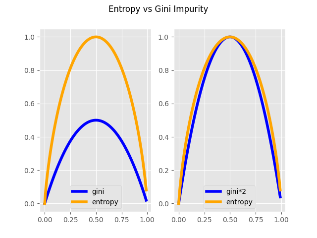
Code to generate plot:
1
2
3
4
5
6
7
8
9
10
11
12
13
14
15
16
17
18
19
20
21
22
23
24
25
26

import numpy as np
import matplotlib.pyplot as plt
import matplotlib
from scipy.stats import entropy

matplotlib.style.use("ggplot")

x_axis = [x for x in np.arange(0, 1, 0.01)]
y_axis_gini = [1 - (x**2 + (1 - x) ** 2) for x in x_axis]
y_axis_gini2 = [x * 2 for x in y_axis_gini]
y_axis_entropy = [entropy([x, 1 - x], base=2) for x in x_axis]

fig, (ax1, ax2) = plt.subplots(1, 2)
fig.suptitle("Entropy vs Gini Impurity")

ax1.plot(x_axis, y_axis_gini, "-", color="blue", linewidth=4, label="gini")
ax1.plot(x_axis, y_axis_entropy, "-", color="orange", linewidth=4, label="entropy")
ax1.legend()

ax2.plot(x_axis, y_axis_gini2, linestyle="-", color="blue", linewidth=4, label="gini*2")
ax2.plot(
    x_axis, y_axis_entropy, linestyle="-", color="orange", linewidth=4, label="entropy"
)
ax2.legend()

plt.show()
Turns out in practice, there is not much difference between using gini and entropy. There are different literatures suggesting computational differences but I have yet to experience a significant example.
Entropy - Continuous
A common area that is not covered - what happens if the predictor X is continuous?
Returning to our example, let’s add weight to our dataset. For the purpose of this example:
- Turns out banana comes in a whole bunches and way heavier $\sim N(150,20)$
- Apple comes second, $\sim N(20,5)$
- Followed by pears, at $\sim N(15,3)$
It should be clear that we will choose a cutoff to filter out all the bananas, right?
Lets generate the dataset:
1
2
3
4
5
6
7
8
9
10
11
12
13
14
15
16
17
18
19
20
21
22
23
24
25
26
27
28
29
30
31

np.random.seed(8888)

WEIGHT_DIST: List[Tuple[float, float]] = [(20.0, 5.0), (150.0, 20.0), (15, 3)]


def assign_weight(input_fruit: str) -> float:
    if input_fruit == "apple":
        # Apple can be red and green
        # but majority of apples are considered red
        x = np.random.normal(WEIGHT_DIST[0][0], WEIGHT_DIST[0][1])
    elif input_fruit == "banana":
        # Banana can be green in color until it is ripe
        # but widely accepted that it is yellow
        x = np.random.normal(WEIGHT_DIST[1][0], WEIGHT_DIST[1][1])
    else:
        # Some pear can be red, yellow, or green - but mostly green
        x = np.random.normal(WEIGHT_DIST[2][0], WEIGHT_DIST[2][1])
    return round(x, 1)


df_weight = df.assign(
    weight=lambda df: df.apply(lambda col: assign_weight(col["target"]), axis=1)
)
df_weight.groupby("target")["weight"].agg(np.mean)

"""
apple      20.075435
banana    146.960714
pear       15.363547
Name: weight, dtype: float64
"""
Turns out, it is pretty straight forward in the case of continuous predictors:
- Take the unique set of values,
- Sort it,
- Find the midpoint of each value
- Calculate the information gain at each midpoint
1
2
3
4
5
6
7
8
9
10
11
12
13
14
15
16
17

all_weights = np.unique(df_weight[["weight"]].values)
all_weights.sort()
results: List[Tuple[float, float]] = []
for i in range(0, len(all_weights) - 1):
    cutoff = 0.5 * (all_weights[i] + all_weights[i + 1])
    IG_cutoff = information_gain(
        df_base=df_weight, logic_input=df_weight["weight"] <= cutoff
    )
    results.append((cutoff, IG_cutoff))

all_info_gain: List[float] = [x[1] for x in results]
which_max: int = all_info_gain.index(max(all_info_gain))
results[which_max]

"""
(57.449999999999996, 0.5929533174474746)
"""
As expected, the information gain of $0.59$ is even better by color split, at approximately $0.46$! In addition, notice the cutoff value of $57.4499$!
Ways to learn
There are multiple ways to learn/built a decision tree, scikit-learn uses an optimised version of the CART algorithm; however, scikit-learn implementation does not support categorical variables for now.
The other approaches can be found in wikipedia, there are:
- ID3 - Iterative Dichotomiser 3
- C4.5 - successor of ID3
- CART - Classification And Regression Tree
- CHAID - Chi-square automatic interaction detection
- MARS - extends decision trees to handle numerical data better.
CART
The Cart algorithm can be summarized as follows:
- Find the best split via gini/entropy (In the case of regression output, by variance reduction or other distance metric, more on that later!)
- Stopping criterion - when a number of
nsamples hit the leaf node - Tree pruning - Prune the tree, the fewer branches the better.
Decision Tree Classifer
Let’s look at some action with sklearn’s decision tree!
Preparing the data:
1
2
3
4
5
6
7
8
9
10
11
12
13
14
15
16
17
18

from sklearn.tree import DecisionTreeClassifier
from sklearn.tree import export_text
from sklearn.preprocessing import LabelEncoder, OneHotEncoder, LabelBinarizer

df_ml = df_weight.copy()
y = df_ml[["target"]]
X = df_ml.drop(["target", "size"], axis=1)
X = pd.get_dummies(X)
X.sample(5)

"""
     weight  color_green  color_red  color_yellow
675   144.3            1          0             0
298    11.0            1          0             0
158    24.6            0          1             0
783    14.7            0          0             1
75     10.1            0          1             0
"""
Now, to fit the tree:
1
2
3
4
5
6
7
8
9
10
11
12
13

decision_tree = DecisionTreeClassifier(random_state=0, max_depth=2)
decision_tree = decision_tree.fit(X, y)
r = export_text(decision_tree, feature_names=list(X.columns))
print(r)
"""
|--- weight <= 57.45
|   |--- color_red <= 0.50
|   |   |--- class: pear
|   |--- color_red >  0.50
|   |   |--- class: apple
|--- weight >  57.45
|   |--- class: banana
"""
As expected,
- Filter by weight to separate banana
- The cutoff is $57.45$ which is same as our previous calculation $57.4499$!
- Then filter by color
Redto separate apples vs pears.
Regression Trees
To use decision tree for regression problems, there is DecisionTreeRegressor! They primarily work the same way,
L2
The L2 error known as the MSE error, and the criteria for L2 regression is as follows,
Given $X_s$, the data $X$ at subset $s$ with mean target value $\bar{y}_s$,
\[H(X_s) = \frac{1}{N_s} \sum_{y\in s} (y-\bar{y}_s)^2\]That is, we want to minimize the error at each node against the mean of each node.
This is equivalent to reduction of variance - which is also what we aim to do in simple linear regression.
L1
Similarly in the case of L1, which is also known as MAE (mean absolute error):
\[H(X_s) = \frac{1}{N_s} \sum_{y\in s} |y- \text{median}(y)_s|\](For those who are interested, L1 regressions estimates median while L2 estimates mean, the explanation is omitted)
Expanded use cases
- Regression trees
- Boosted trees - Incrementally building an ensemble by training each new instance to emphasize the training instances previously mis-modeled
- Bootstrap trees - (or bagged) decision trees, an early ensemble method, builds multiple decision trees by repeatedly resampling training data with replacement, and voting the trees for a consensus prediction.
- Rotation roast - in which every decision tree is trained by first applying principal component analysis (PCA) on a random subset of the input features
References
scikit-learn official docs - decision trees guide
Entropy, Cross-Entropy, and KL-Divergence Explained!
Analytics vidhya - 4 ways to split decision trees
Extra notes on using decision trees - towardsdatascience
Geeksforgeeks - Gini impurity vs entropy