CS7643 OMSCS - Deep Learning Notes
Content of these notes are from Georgia Tech OMSCS 7643: Deep Learning by Prof. Zsolt Kira. They kindly allowed this to be shared publicly, please use them responsibly!
Module 1: Introduction to Neural Networks
Lesson 1: Linear Classifiers and Gradient Descent
Readings
- DL book: Linear Algebra background
- DL book: Probability background
- DL book: ML Background
- LeCun et al., Nature ‘15
- Shannon, 1956
Performance Measure
For a binary classifier:
\[y = \begin{cases} 1, & \text{if $f(x,w)$ > 0} \\ 0, & \text{otherwise} \end{cases}, f(x,W) = W * x + b\]But we often want probabilities, we can use softmax:
\[s = f(x,W) \tag{Scores}\] \[P(Y=k|X=x) = \frac{e^{s_k}}{\sum_j e^{s_j}} \tag{Softmax}\]We need a performance measure to optimize known as the objective or loss function. Given a set of examples ${(x_i,y_i)}^{N}_{i=1}$, the loss can be defined as:
\[L = \frac{1}{N} \sum L_i (f(x_i,W),y_i)\]For example, the SVM loss has the form:
\[\begin{aligned} L_i &= \sum_{j\neq y_i} \begin{cases} 0, & \text{if $s_{y_i} \geq s_j +1$} \\ s_j - s_{y_i} + 1, & \text{otherwise} \end{cases} \\ &= \sum_{j\neq y_i} max (0, s_j - s_{y_i} + 1) \end{aligned}\]For a particular data point $x_i, y_i$, if the model is accurate, then $s_{y_i}$ will be large and $s_j$ will be small. This will make $max (0, s_j - s_{y_i} + 1)$ be equal to 0 (there is no loss). This is called a hinge loss.
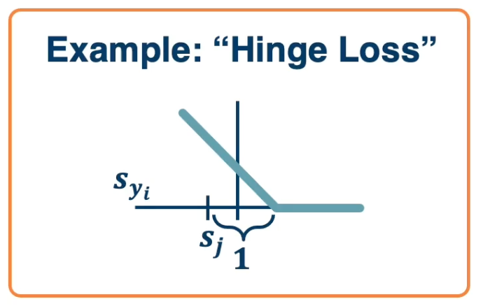
For example:
| cat | 3.2 | 1.3 | 2.2 |
| car | 5.1 | 4.9 | 2.5 |
| frog | -1.7 | 2.0 | -3.1 |
In the case of the cat:
\[\begin{aligned} L_{cat} &= \sum_{j\neq y_i} max (0, s_j - s_{y_i} + 1) \\ &= max(0,5.1-3.2+1) + max(0, -1.7, -3.2 + 1) \\ &= max(0,2.9 ) + max(0, -3.9) \\ &= 2.9 + 0 \\ &= 2.9 \end{aligned}\]We can see that in this case the model thinks that the car is most likely even though the truth is cat. This contributed a loss of 2.9. In the case of cat versus frog, there is a score of 0 since the model thinks it is most likely a cat instead of a frog.
If we use the softmax function to convert scores to probabilities, the right loss function to use is cross entropy:
\[L_i = - log P(Y=y_i|X=x_i)\]This can be derived from various ways:
- KL divergence - looks at distance between two probability distributions.
- Maximum Likelihood Estimation - Choose probabilities to maximize the likelihood of the observed data.
Back to the cat example:
\[\underbrace{\begin{pmatrix} 3.2 \\ 5.1 \\ -1.7 \end{pmatrix}}_{\text{Unnormalized logits}} \overset{\mbox{exp}}{\longrightarrow} \underbrace{\begin{pmatrix} 24.5 \\ 164 \\ -0.18 \end{pmatrix}}_{\text{Unnormalized probabilities}} \overset{\mbox{normalize}}{\longrightarrow} \underbrace{\begin{pmatrix} 0.13 \\ 0.87 \\ 0.00 \end{pmatrix}}_{\text{Normalized probabilities}}\]So, $L_{cat} = - log(0.13)$.
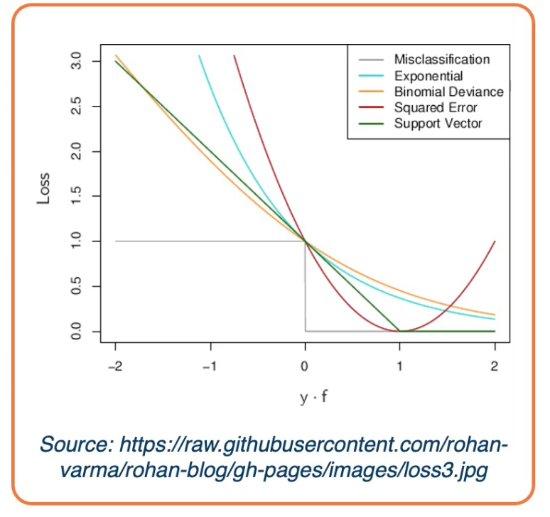
There are other forms of loss functions, such as:
In the case of a regression problem:
- L1 loss : $L_i = |y-Wx_i|$
- L2 loss : $L_i = |y- Wx_i|^2$
For probabilities:
- Logistics: $L_i = |y-Wx_i| = \frac{e^{s_k}}{\sum_j e^{s_j}}$
We can also add regularization to the loss function to prefer different models over others based on the complexity of the model. For example in L1 regularization: $L_i = |y-Wx_i|^2 + |W|$.
Linear Algebra View
\[W = \begin{bmatrix} w_11 & w_12 & ... & w_1m & b1 \\ w_21 & w_22 & ... & w_2m & b2 \\ & & \ddots & & \\ w_c1 & w_c2 & ... & w_cm & bc \\ \end{bmatrix}_{c \times (d+1)}, X = \begin{bmatrix} x_1 \\ x_2 \\ \vdots \\ x_m \\ 1 \end{bmatrix}_{(d+1) \times 1}\]Where:
- $c$ is the number of classes
- $d$ is the dimensionality of input
Conventions:
- size of derivatives for scalars, vectors and matrices:
Assume we have scalar $s \in \mathbb{R}^1$, vector $v \in \mathbb{R}^m$ i.e. $v = [v_1, v_2, …, v_m]^T$ and matrix $M \in \mathbb{R}^{k \times l}$, - What is the size of $\frac{\partial v}{\partial s}$?
- $\mathbb{R}^{m\times 1}$ - column vector of size m $[\frac{\partial v_1}{\partial s}, … , \frac{\partial v_m}{\partial s}]^T$
- What is the size of $\frac{\partial s}{\partial v}$?
- $\mathbb{R}^{1\times M}$ - row vector of size m $[\frac{\partial s}{\partial v_1}, … , \frac{\partial s}{\partial v_m}]$
- What is the size of $\frac{\partial v^1}{\partial v^2}$?
- A matrix called a Jacobian with each index as $\frac{\partial v_i^1}{\partial v_j^2}$
- What is the size of $\frac{\partial s}{\partial M}$
- A Matrix with each index as $\frac{\partial s}{\partial m_{[i,j]}}$
- all the elements in the matrix essentially give sus the partial derivastive of the scalar with respect to each element in the matrix.
- What is the size of $\frac{\partial L}{\partial W}$? Note, this is the partial derivative of the loss with respect to the weights W.
- Remember that loss is a scalar and W is a matrix, and the Jacobian is also a matrix, thus:
As mentioned, gradient descent works in batches of data. These are referred to as matrices or tensors (multi-dimensional matrices)..
Examples:
- Each instance of a vector of size m, our batch is of size $[B\times m]$
- Each instance is a matrix (e.g grayscale image) of size $W \times H$, our batch is $[B \times W \ times H]$
- Each instance is a multi-channel matrix (e.g color image with RGB channels) of size $C \times W \ times H$, our batch is $[B \times C \times W \times H]$
Jacobians becomes tensors which is complicated
- Instead, flatten input into a vector and get a vector of derivatives.
- This can also be done for partial derivatives between two vectors, two matrices or two tensors.
Gradient descent
Given a model and loss function, finding the best set of weights is a search problem, which is to find the best combination of weights that minimizes our loss function. Several classes of methods can be used:
- Random Search
- Genetic Algorithms (population-based search)
- Gradient-based optimization
In deep learning, gradient-based methods are dominant although not the only approach possible.
The key idea is as weights change, the loss changes as well. We cna therefore think about iterative algorithms that can take the current values of weights and modify them a bit.
The derivative is defined by
\[f'(a) = lim_{h \rightarrow 0} \frac{f(a+h)-f(a)}{h}\]Intuitively, steepest descent direction is the negative gradient and intuitively measures how the function changes as the argument a changes by a small step size. In machine learning we want to know how the loss function changes as weights Are varied. We can consider each parameter separately by taking partial derivative of loss function with respect to that parameter.
This idea can be turned into an algorithm (gradient descent)
- Choose a model: $f(x,W) = Wx$
- Choose loss function: $L_i = |y-Wx_i|^2$
- Calculate partial derivative for each parameter: $\frac{\partial L}{\partial w_j}$
- Update the parameters: $w_j = w_j - \frac{\partial L}{\partial w_j}$
- Add learning rate to prevent too big of a step: $w_j = w_j - \alpha \frac{\partial L}{\partial w_j}$
Often, we only compute the gradients across a small subset of data
- Full Batch Gradient Descent: $L = \frac{1}{N}\sum L(f(x_i,W),y_i)$
- Mini-Batch Gradient Descent $L = \frac{1}{M}\sum L(f(x_i,W),y_i)$
- Where $M$ is a subset of data
- We iterate over mini-batches
- Get mini-batch, compute loss, compute derivatives, and take a step. The mini-batch can be sampled randomly or taken iteratively.
- Another thing to note we often average the loss across the mini batches and therefore your gradients also get averaged across the size of the mini batch.
- This is to prevent large changes in the learning rate if your batch size changes, so if you choose a batch size of 32 examples to calculate the loss over, but then the next day choose 128 examples, then you’ll be taking much larger steps and you’ll have to change the learning rate or tune their learning rate again.
Gradient descent is guaranteed to converge under some conditions:
- For example, learning rate has to be appropriately reduced throughout training
- It will converge to a local minima
- small changes in weights would not decrease the loss
- It turns out that some of the local minima that it finds in practice (if trained well) are still pretty good!
We know ow to compute the model output and loss function and there are several ways to compute $\frac{\partial L}{\partial w_i}$:
- Manual differentiation
- Often labour intensive and in some cases cannot really compute the closed form solution.
- Symbolic differentiation
- Only work for some classes of functions and is also labour intensive
- Numerical differentiation
- Can do for any function but it is very computationally intensive.
- Automatic differentiation
- Deep learning frameworks mostly use automatic differentiation
An Example:
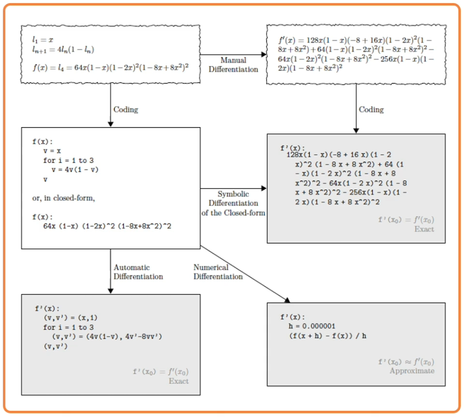
For some functions, we can analytically derive the partial derivative, example:
\[f(w,x_i) = w^T x_i, Loss = (y_i-w^Tx_i)^2\]Assume $w$ and $x_i$ are column vectors, so same as $w \cdot x_i$. Then the update rule:
\[\begin{aligned} w_j &= w_j - \eta \frac{\partial L}{\partial w_j }\\ &= w_j + 2\eta \sum_{i=1}^N (y_i - w^T x_i) x_{ij} \end{aligned}\]Proof:
\[\begin{aligned} L &= \sum_{i=1}^N (y_i - w^T x_i)^2 \\ \frac{\partial L}{\partial w_j} &= \sum_{i=1}^N \frac{\partial}{\partial w_j} (y_i - w^T x_i)^2 \\ &= \sum_{i=1}^N 2(y_i - w^T x_i)\frac{\partial}{\partial w_j}(y_i - w^T x_i) \\ &= -2 \sum_{i=1}^N (y_i - w^T x_i) \frac{\partial}{\partial w_j}(w^T x_i) \\ &= -2 \sum_{i=1}^N (y_i - w^T x_i) \frac{\partial}{\partial w_j} \sum_{k=1}^m w_kx_{ik} \\ &= -2 \sum_{i=1}^N (y_i - w^T x_i) x_{ij} \end{aligned}\]If we add a non linearity (sigmoid), derivation is more complex:
\[\begin{aligned} \sigma(x) &= \frac{1}{1+e^{-x}} \\ \sigma'(x) &= \sigma(x)(1-\sigma(x)) \end{aligned}\]Then:
\[\begin{aligned} f(x) &= \sigma \bigg(\sum_k w_kx_k \bigg) \\ L &= \sum_i \bigg( y_i - \sigma \big(\sum_k w_kx_k \big)\bigg)^2 \\ \frac{\partial L}{\partial w_j} &= 2 \sum_i \bigg( y_i - \sigma \big(\sum_k w_kx_k \big)\bigg)\bigg( -\frac{\partial}{\partial w_j} \sigma\bigg( \sum_k w_k x_{ik}\bigg)\bigg) \\ &= -2 \sum_i \bigg( y_i - \sigma \big(\sum_k w_kx_k \big)\bigg)\sigma'\bigg(\sum_k w_k x_{ik}\bigg) \frac{\partial}{\partial w_j} \sum_k w_kx_{ik}\\ &= \sum_i -2\delta_i \sigma(d_i)(1-\sigma(d_i))x_{ij} \end{aligned}\]where:
- $\sigma_i = y_i-f(x_i)$
- $d_i = \sum w_kx_{ik}$
So the sigmoid perception update rule:
\[\begin{aligned} w_j &= w_j + 2\eta \sum_{i=1}^N \delta_i \sigma_i (1-\sigma_i)x_{ij} \\ \sigma_i &= \sigma \bigg( \sum_{k=1}^m w_kx_{ik}\bigg) \\ \delta_i &= y_i - \sigma_i \end{aligned}\]Now if you noticed, even analytically deriving the partial derivative of the loss with respect to particular parameters, for a pretty simple simple function, a sigmoid of a linear function is actually not that nice. Wht we want to do is rather than have to by hand derive this partial derivative, we are going to try to simplify the problem. We are going to decompose the complicated function into modular sub blocks, and this will allow us to develop a generic algorithm that can work on these sub blocks to derive the partial derivative.
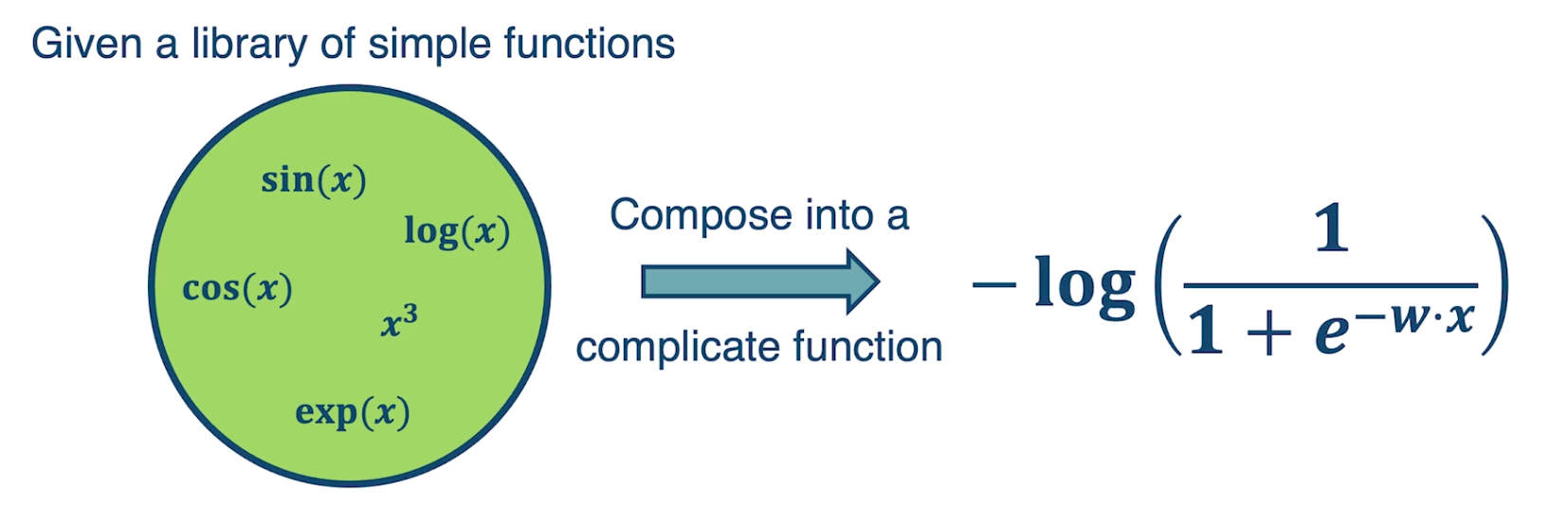
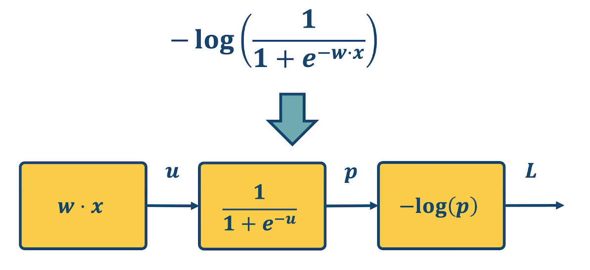
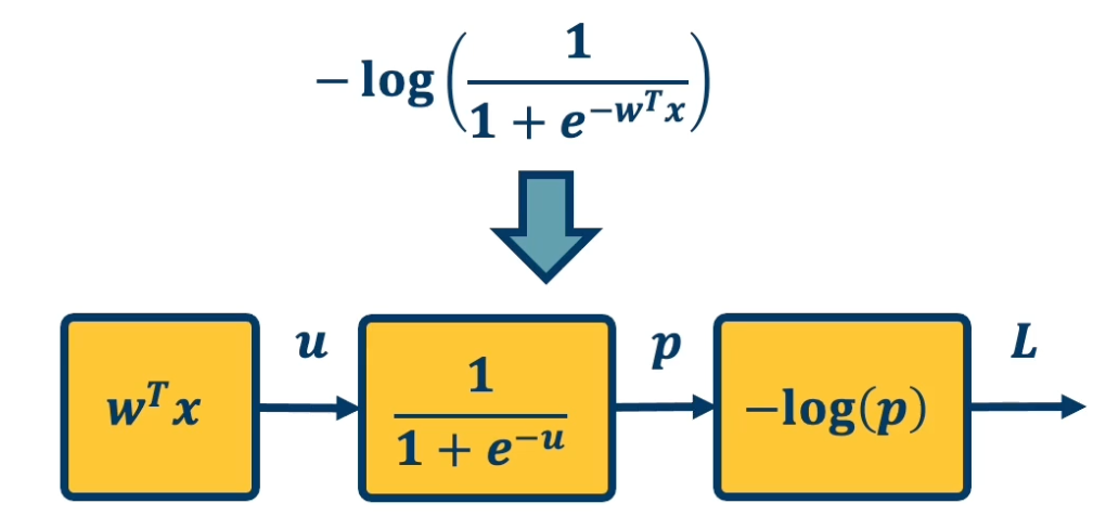
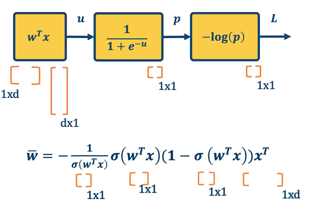
So given a library of simple functions, including addition, subtraction, multiplication, sin, cosin, log and exponential, we are going to compose it into a more complicated function, for example negative log of sigmod function. This is just the typical logistic machine learning algorithm and so what we are going to do is decompose that complex function into a set of modular sub blocks.
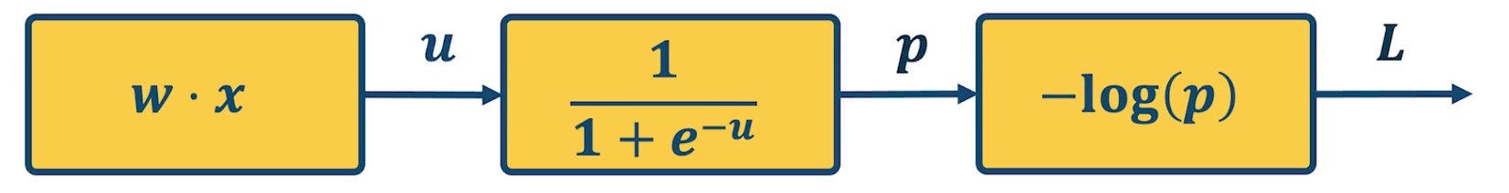
Under the left side, we have the innermost part of the function, w transpose x, that gets output into an intermediate variable u, which goes into the next sub block which is, again the logistic or sigmoid function. That gets output into another immediate variable p, and then we compute the negative log of p, which is our loss function and that is the final output of the model.
This will allow us to develop a generic algorithm to perform the differentiation that we want which is the partial derivative of the loss with respect to intermediate variables here. For example we may want the partial derivative of the loss with respect to $u$, or at the end we want the partial derivative of the loss with respect to $w$ because that is ultimately what gradient descent wants to update.
How is deep learning different?
Hierarchical Compositionality
- Cascade of non-linear transformations
- Multiple layers of representations
For example:
This can be done by linear combinations $f(x) = \sum_i \alpha_i g_i (x)$ or composition functions $f(x) = g_1(g_2(…(g_n(x))))$. They key is we can use any of this as long as the function is differentiable.
End-to-End learning
- Learning (goal-driven) representations
- Learning feature extraction
Entire spectrum from raw data to feature extraction to classification.
Distributed Representations
- No single neuron “encodes” everything
- Groups of neurons work together
Lesson 2: Neural Networks
Readings
- DL book: Deep Feedforward Nets
- Automatic Differentiation Survey, Baydin et al.
- Matrix calculus for deep learning
Neural Network View of a linear classifier
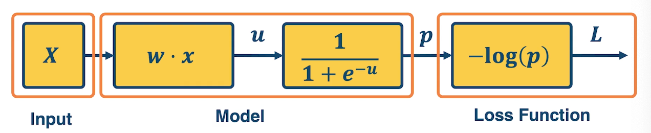
A linear classifier can be broken down into:
- input
- a function of the input
- a loss function
It is all just one function that can be decomposed into building blocks:
A simple neural network has similar structure as our linear classifier:
- A neuron takes inputs (firing) from other neurons (-> input into linear classifier)
- The inputs are summed in a weighted manner (-> weighted sum)
- Learning is through a modification of the weights (gradient descent in the case of NN)
- If it receives enough inputs, it “fires” (if it exceeds the threshold or weighted sum plus bias is high enough)
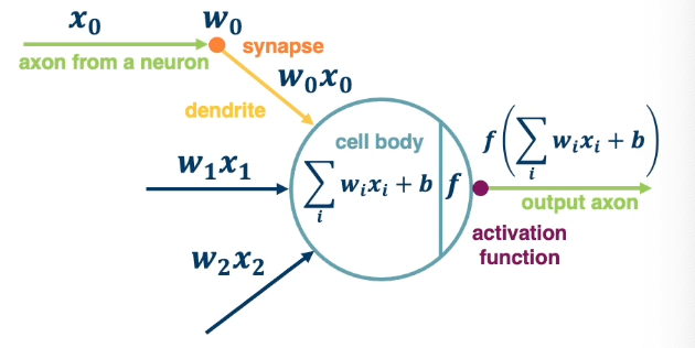
The output of a neuron can be modulated by a non linear function (e.g sigmoid).
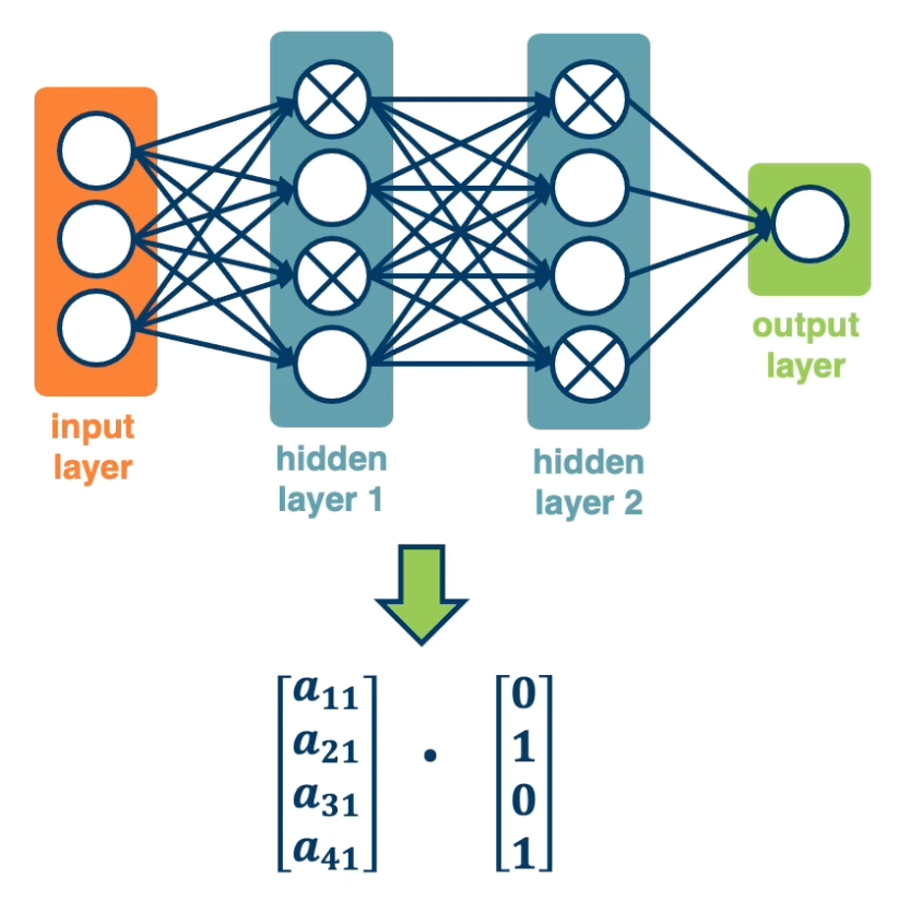
We can have multiple neurons connected to the same input:
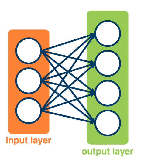
Note, often in these visual depictions, you do not see the activation function. it is assumed that each node in the output layer contains both the weighted sum and the sigmoid activation.
- Each output node outputs the score for a class. \(f(x,W) = \sigma(Wx+b) = \begin{bmatrix} w_{11} & w_{12} & \cdots & w_{1m} & b_1 \\ w_{21} & w_{22} & \cdots & w_{2m} & b_2 \\ w_{31} & w_{32} & \cdots & w_{3m} & b_3 \\ \end{bmatrix}\)
- Often called fully protected layers (also called a linear projection layer)
- Each input/output is a neuron (node)
- A linear classifier is called a fully connected layer.
- Connections are represented as edges
- Output of a particular neuron is referred to as activation
- This will be expanded as we view computation in a neural network as a graph.
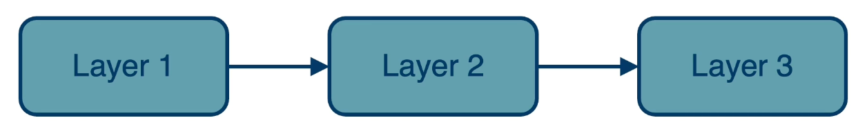
With this, it is possible to stack multiple layers together where the input of the second layer is the first layer. The middle layers are also known as hidden layers and will see that they end up learning effective features. This increases the representation power of the function, and two layered networks can represent any continuous function.
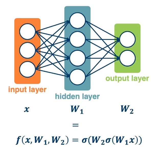
The same two layered neural network corresponds to adding another weight matrix, as seen above as $W_1$ and $W_2$. Large (deep) networks can be built by adding more and more layers, and three-layer networks can represent any function.
- However, the number of nodes could grow unreasonably (Exponential or worse) with respect to the complexity of the function.
- So it is not clear how to learn such a function and the weights, as well as the architecture of the neural network.
Computation Graph
Our goal is to generalize our viewpoint of multi-layered neural networks as computation graphs. Functions can be made arbitrarily complex (subject to memory and computational limits).
\[f(x,W) = \sigma(W_5\sigma(W_4\sigma(W_3\sigma(W_2\sigma(W_1x)))))\]We can use any time of differentiable function (layer) as well. The reason to use a differentiable function is to be able to use gradient descent to optimize these functions. At the end, add the loss function.
Composition can have some structure! Empirical and theoretical evidence that it makes learning complex functions easier. Note that prior state of the art engineered features often had this compositionality as well.
The key with deep learning is to employ this compositionality through the architecture of the neural network.
- we are learning complex models with significant amount of parameters (millions or billions).
- If so, how do we compute the gradients of the loss (at the end) with respect to internal parameters?
- Intuitively, want to understand how small changes in weight deep inside Are propagated to affect the loss function at the end.
To develop a general algorithm for this, we will view the function as a computation graph. Graph can be any directed acyclic graph (DAG); it can have any structure as long as there are no cycles.
- Modules must be differentiable to support gradient computations for gradient descent.
A *training algorithm** will then process this graph, one module at a time, to calculate the singular value that we want, which is the change in loss with respect to parameters of that module.
Here is an example of the computational graph notion (note that this might not be the only possible representation):
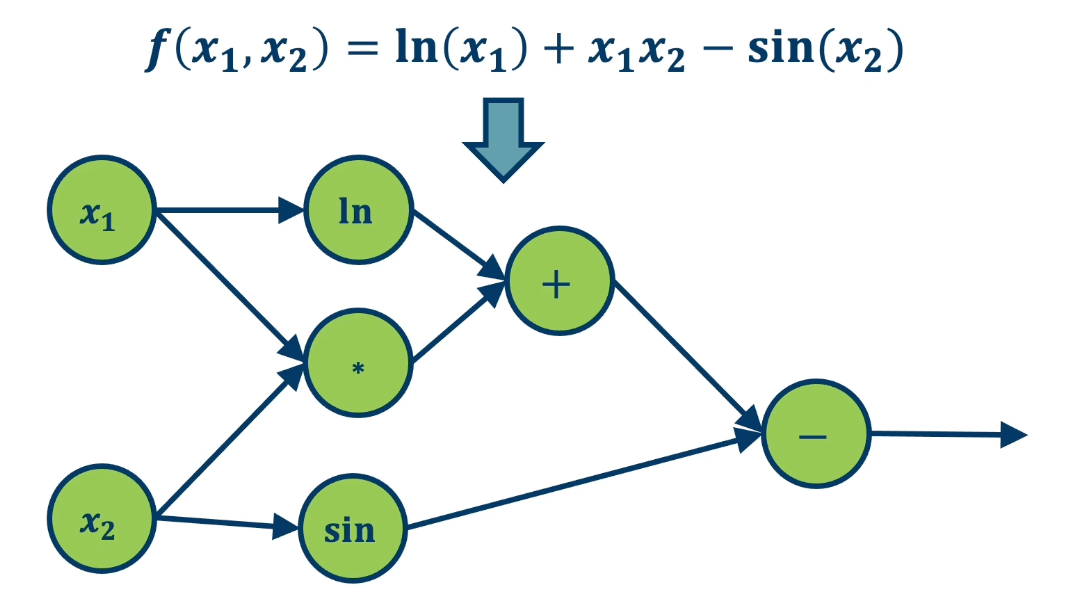
- The function $f(x_1,x_2) = ln(x_1) + x_1 x_2 - sin(x_2)$ as a graph*
The most important thing are the edges so that we know which order when we compute the function forward.
To repeat, any arbitrarily complex function can be decomposed in this manner and this will become clear in the next few lessons.
Backpropagation
Backpropagation allows us to compute the important gradient information that we need for gradient descent when we have a deep neural network.
Given this computation graph, where we decompose a complicated function into its constituent parts, the training algorithm will perform the following computation:
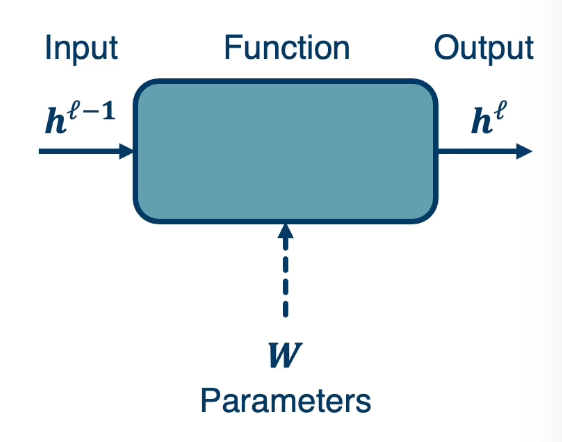
- Calculate the current model’s output (called the forward pass)
- So in the diagram, will feed in the input of $h^{\ell-1}$ which is the layer before this model. Then will compute whatever function that this modules performs. For example $W^Tx$ and so it could have some parameters. Although note that some modules may not have any any parameters. Then we will be able to compute $h^\ell$ which is the output of this module.
- Calculate the gradients for each module (called the backward pass)
The backward pass is a recursive algorithm that:
- Start at loss function where we know how to calculate the gradients. (We seen examples in Lesson1)
- Progresses back through the modules. We do this by passing back key pieces of information in the form of gradients.
- Ends in the input layer where we do not need gradients (no parameters)
 Note, sometimes we call them modules, sometimes layers.
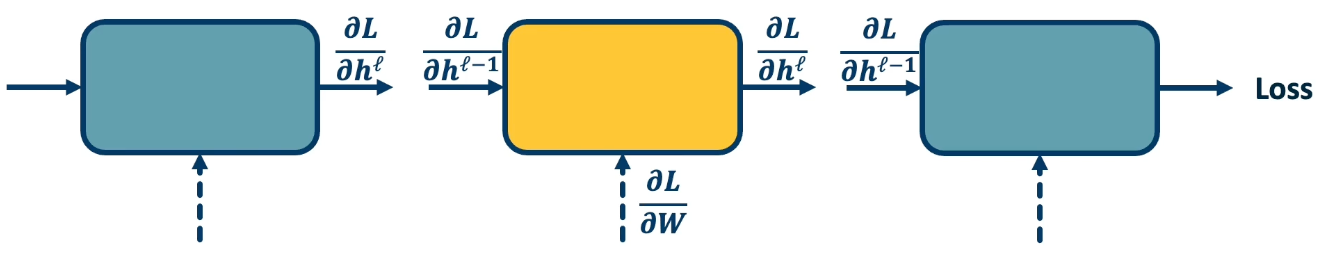
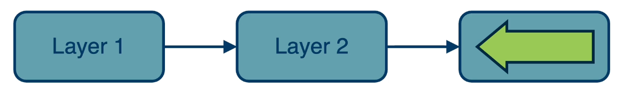
Forward Pass (Step 1)
First, compute loss on mini-batch: forward pass
- E.g calculate L1, pass the output to L2, and repeat again to L3.
- Note that we must store the intermediate outputs of all layers because we will need it in the backwards computation to compute the gradients
- The gradient equation will have terms with the output values in them.
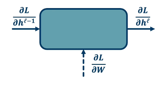
In the backward pass, we seek to calculate the gradients of the loss with respect to the module’s parameters. So take a generic module any point in the computation graph, we will have three different terms here.
- Partial derivative of the loss with respect to the input of the module $\frac{\partial L}{\partial h^{\ell -1}}$
- Partial derivative of the loss with respect to our output, $\frac{\partial L}{\partial h^{\ell}}$
- Partial derivative of the loss with respect to our weights: $\frac{\partial L}{\partial W}$
For gradient descent, this is the key thing that we need, we need to know how the loss changes, no matter where it is. A particular module may not be connected to that loss function, it may go through a whole series of other modules afterwards and then be connected to a loss function. But we still need to know in the end, how the loss will change at the end if we change our parameters within this module.
- We are going to assume in this recursive algorithm is that we have the gradient of the loss with with respect to the module’s outputs (given to us by upstream module). This is the change in loss with respect to $h^\ell$
- Also going to pass the gradient of the loss with respect to the module’s input.
- This is not required for update the module’s weights, but passes the gradients back to the previous module. (This is really just passing back information so the previous layer also can calculate this gradient)
Problem:
-
We can compute the local gradients as the input changes or the change in output as the weights change. This is because we know the actual function this module computes, for example $W^Tx$.
\[\bigg\{ \frac{\partial h^\ell}{\partial h^{\ell-1}}, \frac{\partial h^\ell}{\partial W} \bigg\}\] - We are given: $\frac{\partial L}{\partial h^\ell}$
- This is from the assumption
-
Compute the change in loss with respect to our weights in order to perform gradient descent and take a step in the weights. In other words, update the weight through the negative gradient. We also need to compute the change in loss with respect to our inputs. This is not required for the gradient descent update for this particular module but it is required so we can pass this gradient to the previous module.
\[\bigg\{ \frac{\partial L}{\partial h^{\ell-1}}, \frac{\partial L}{\partial W} \bigg\}\]
Recall that we can compute the local gradients $\{ \frac{\partial h^\ell}{\partial h^{\ell-1}}, \frac{\partial h^\ell}{\partial W} \}$. This is just the derivative of our function with respect to its parameters and inputs!
For example, if $h^\ell = Wh^{\ell-1}$, then $\frac{\partial h^\ell}{\partial h^{\ell-1}} = W$ and $\frac{\partial h^\ell}{\partial W} = {h^{\ell-1}}^T$.
Now, we want to compute: $\{ \frac{\partial L}{\partial h^{\ell-1}}, \frac{\partial L}{\partial W} \}$, we need to use chain rule!
Zooming in to the particular module:
Gradient of loss w.r.t. inputs: $\frac{\partial L}{\partial h^{\ell-1}} = \underbrace{\frac{\partial L}{\partial h^\ell}}_{\text{given}} \frac{\partial h^\ell}{\partial h^{\ell-1}}$
Gradient of loss w.r.t. weights: $\frac{\partial L}{\partial W} = \frac{\partial L}{\partial h^\ell} \frac{\partial h^\ell}{\partial W}$
Backward Pass (Step 2)
We start at the loss function where we actually know how to compute the gradient of the loss with respect to this module. This is just the exercise that we did earlier where we had a classifier that is directed connected to the loss. We just compute the change in loss with respect to the inputs of the function or with respect to the parameters. So we will compute the gradients with respect to the parameters to perform gradient descent and then we will compute the gradient of the loss with respect to our inputs in order to send this back to the previous layer.
And now the previous layer knows how the loss changes if its output changes and it uses the chain rule to compute how does the loss change if our inputs change, and how does the loss change if our weights or parameters change. Similarly, it will then pass back that upstream gradient to the first layer.
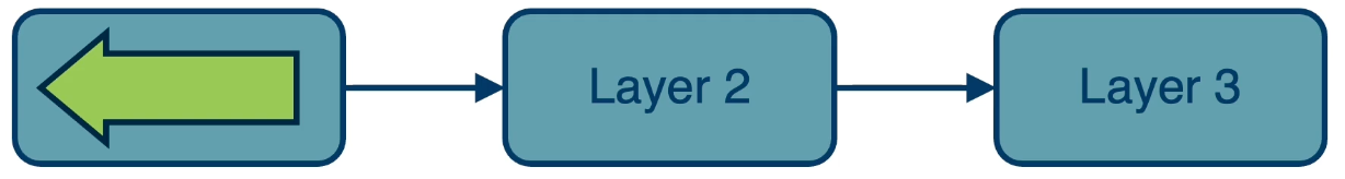
And again, the first layer can compute the change in loss way at the end of the computation graph with respect to its own parameters. In this case, it does not really need to send back any gradients because there is no previous layer.
Update all parameters (step 3)
Use gradient to update all parameters at the end.
And then, once we have these terms the change in loss with respect to all the weights for all the layers, we are just going to use gradient descent. We pdate the weights by subtracting the gradient going into the negative gradient direction multiplied by some learning rate.
\[w_i = w_i - \alpha \frac{\partial L}{\partial w_i}\]So, Backpropagation is just the application of gradient descent to a computation graph via the chain rule.
Backpropagation and Automatic Differentiation
Backpropagation tells us to use the chain rule to calculate the gradients, but it does not really spell out how to efficiently carry out the necessary computations. But the idea can be applied to any directed acyclic graph (DAG).
- Graph represents an ordering constraining which paths must be calculated first.
Given an ordering, we can then iterate from the last module backwards, applying the chain rule.
- We will store, for each node, its gradient outputs for efficient computation
- Such as the activations for the forward pass as well as the gradient outputs.
This is called reverse-mode automatic differentiation
- The key idea here is that we will decompose the function into very simple primitive functions where we already know what the derivatives are.
Computation = Graph
- Input = Data + Parameters
- Output = loss
- Scheduling = Topological ordering (defined by the graph)
Auto-Diff (Auto differentiation)
- A family of algorithms for implementing chain rule on computation graphs.
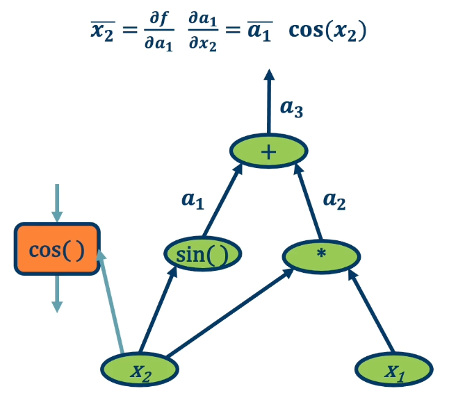
An example:
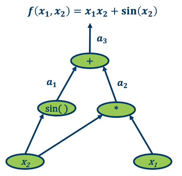
We want to find the partial derivative of output f with respect to all intermediate variables.
- Assign some intermediate variables such as $a_1 = sin(x_2)$ and $a_2 = x1 \times x2$ and $a_3$ is the final output.
- To simplify notation, denote $\bar{a_3} = \frac{\partial f}{\partial a_3}$
- In gradient descent as well as in these examples, you want the partial derivative of the output, the final output of the function with respect to all the intermediate variables. The intermediate variables in a machine learning computation graph will be the weight matrices.
- Start at the end and move backwards.
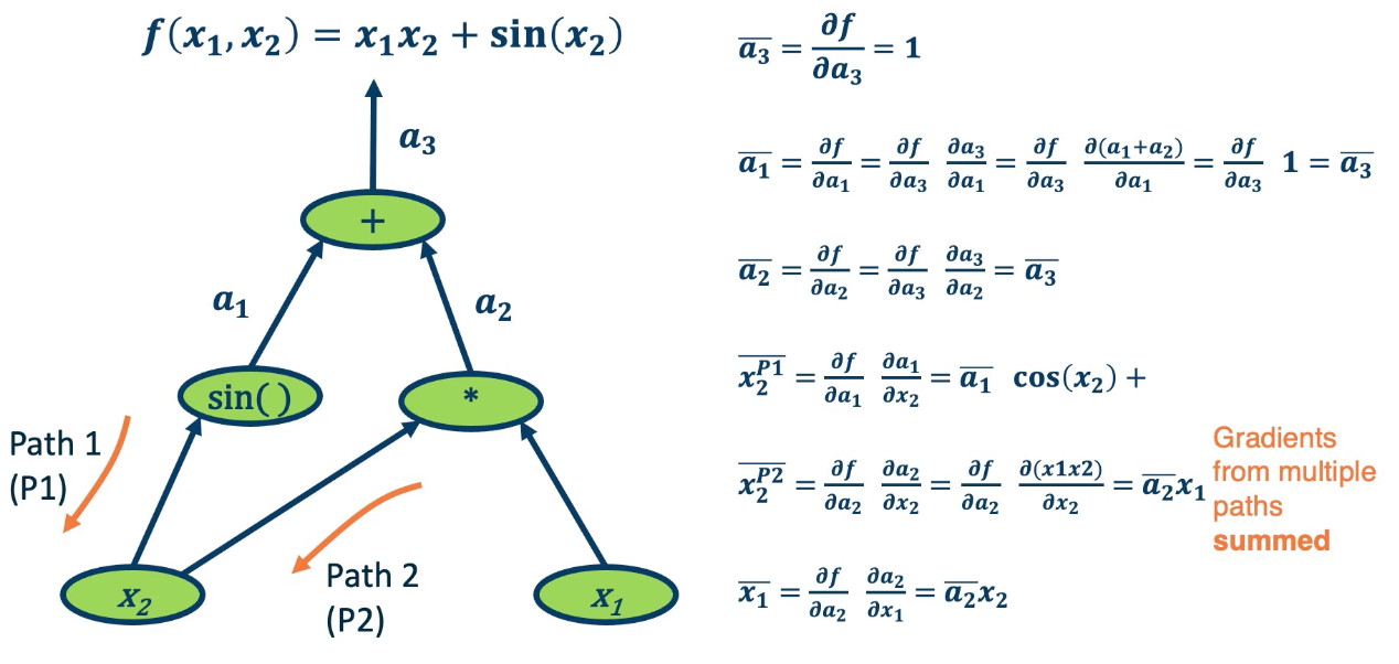
One thing to note is gradient from multiple paths have to be accounted for, and the way we do this is by just summing them up together. So in the case of $\bar{x_2}$ there is path 1 and path 2. This makes intuitive sense since if we want to understand how the change in $x_2$ affects the final output of the function, we need to basically propagate it across all paths that occur from it to that function.
One interesting thing that we can notice as we analyze this is that different operations have different effects on the gradient.
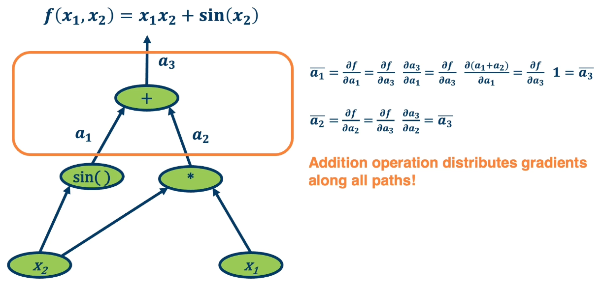
For example, in the addition operation, we will notice that $\bar{a_1}$ and $\bar{a_3}$ is the same. This is because the plus operation is actually a gradient distributor. It takes the partial derivative of $f$, the function output with respect to it and distributes it back across all the paths.
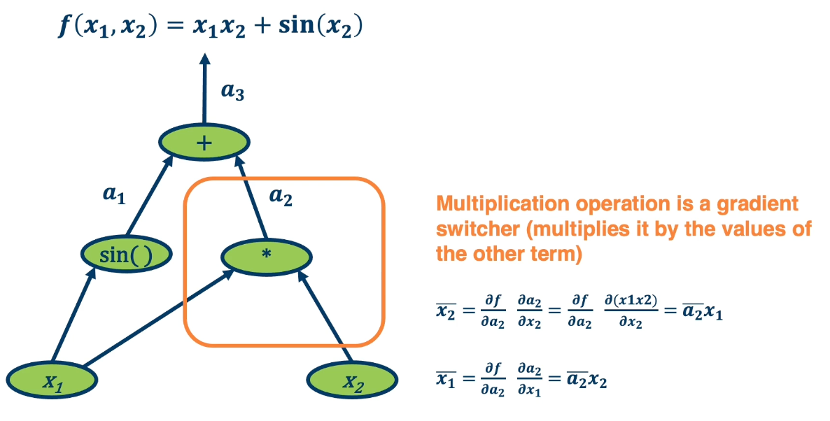
Multiplication, on the other hand, does something different with the gradients. $\bar{x_2} = \bar{a_2}x_1$. So it is the upstream gradient times the other inputs. Where else $\bar{x_1} = \bar{a_2}x_2$ which is the same thing but in reverse. So multiplication operation is a gradient switcher, it multiplies it by the value of the other term.
Why is this important? Gradients are the key things that gradient descent work on. If the gradients have a particular property such as they become too small or become degenerate, then learning will not happen. So one of the key considerations that we will use as we design these computation graphs for machine learning is how gradients flow back through the entire computation graph or model that we will have. This is a key piece of information that we will want to analyze and understand in order to ensure that the model is going to be learning properly.
There are several other patterns as well,
- The gradient is passed back through the original path taken*
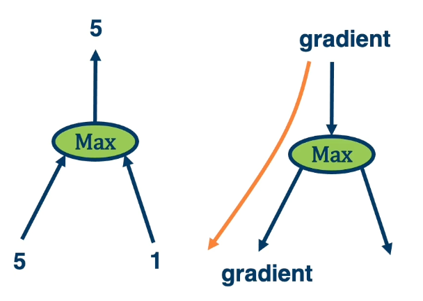
Max operation selects which path to push the gradients through.
- Gradient flows along the path that was “selected” to be the max
- This information must be recorded in the forward pass.
The flow of gradients is one of the most important aspects in deep neural networks. So for example in the example of $max(5,1) = 5$, we need to remember we used the left side. So when we pass back the gradient, we only pass through that particular element that was selected to be the maximum.
- If the gradients do not flow backwards properly, learning slows or stops!
Key Idea
- Key idea is to explicitly store computation graph in memory and corresponding gradient functions. For example the derivative of sine is cosine.
- Nodes broken down to basic primitive computations (addition, multiplication, log, …) for which corresponding derivative is known.
Forward mode automatic differentiation
There is also something called forward mode automatic differentiation. This is computing exactly the same terms that we want, which is the partial derivative of the function output with respect to all the intermediate variables. Unlike reverse mode automatic differentiation that has a forward pass and backward pass. Here we start from inputs and propagate gradients forward. So we have many forward passes one for each input. The complexity is proportional to input size because run forward across each input.
In deep learning, most of the times inputs (images) are large and outputs (loss) are small.
One of the powerful things about automatic differentiation is it allows deep learning frameworks to basically build out these computation graphs as we code. So frameworks like pytorch runs this generic algorithm that works on any computation graph.
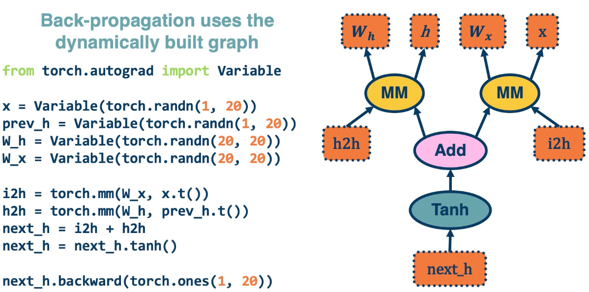 This is an older version of pytorch which is more complex
The last line computes the backwards gradient all in one line of code.
- Computation graphs are not limited to mathematical functions
- Can have control flows (if statements, loops) and backpropagate through algorithms!
- Can be done dynamically so that gradients are computed, then nodes are added, repeat.
- Concept is called differentiable programming
Computation Graph example for logistic regression
- Input $x \in \mathbb{R}^D$
- Binary label $y \ in \{-1,+1\}$
- Parameters $w \in \mathbb{R}^D$
- Output prediction: $p(y=1|x) = \frac{1}{1+e^{-w^Tx}}$
- Loss $L = \frac{1}{2} \lVert w \rVert^2 - \lambda log(p( y \lvert x))$
where $p = \sigma(w^Tx)$ and $\sigma(x) = \frac{1}{1+e^{-x}}$
\[\begin{aligned} \bar{u} &= \frac{\partial L}{\partial u} = \frac{\partial L}{\partial p}\frac{\partial p}{\partial u } = \bar{p}\sigma(w^Tx)(1-\sigma(w^Tx))\\ \bar{p} &= \frac{\partial L}{\partial w} = \frac{\partial L}{\partial u}\frac{\partial u}{\partial w} = \bar{u}x^T \end{aligned}\]We can do this in a combined way to see all the terms together:
\[\begin{aligned} \bar{p} &= \frac{\partial L}{\partial p} \frac{\partial p}{\partial u}\frac{\partial u}{\partial w}\\ &= - \frac{1}{\sigma(w^Tx)} \sigma(w^Tx)(1-\sigma(w^Tx))x^T \\ &= - (1-\sigma(w^Tx))x^T \end{aligned}\]This effectively shows the gradient flow along path from $L$ to $w$
Vectorization and Jacobians of simple layers
The chain rule can be computed as a series of scalar, vector, and matrix linear algebra operations. These are extremely efficient in graphics processing units (GPU).
Lets take a look at specific neural network layer types and see what their matrices and vectors look like as well as the resulting gradients or jacobian. This is also the simple fully connected linear layer.
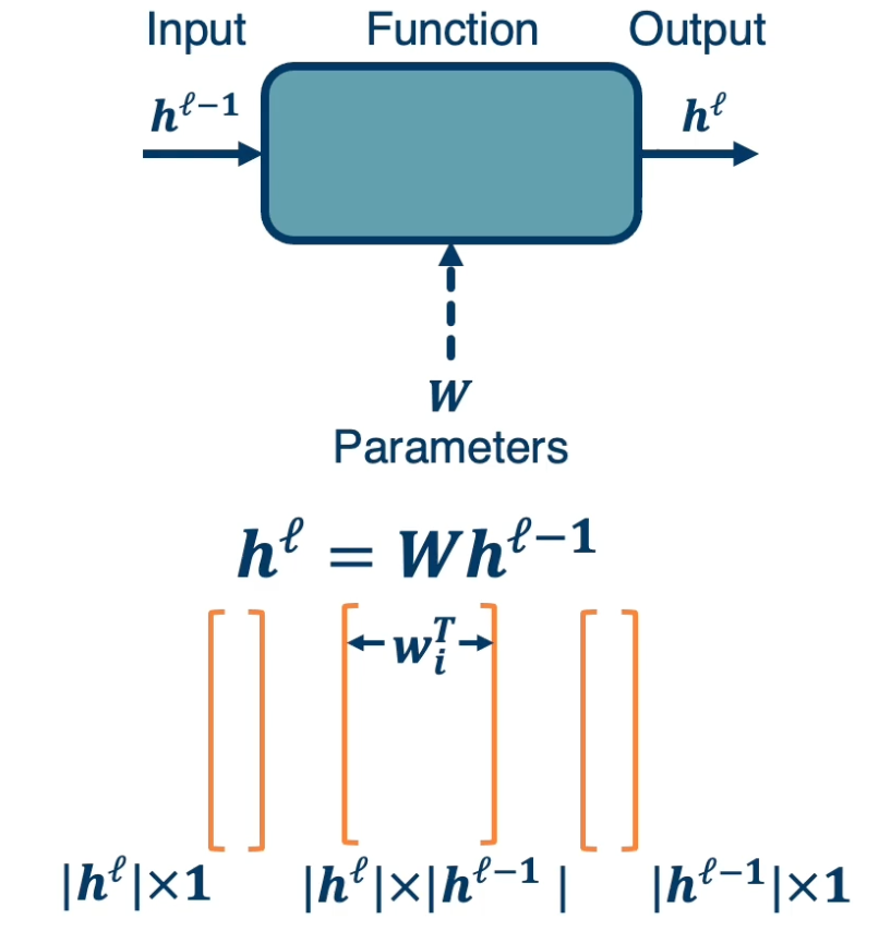
We have $h^\ell = Wh^{\ell-1}$ which is the previous layer multiplied by $w$.
- $h^\ell$ has dimension $\lvert h^\ell \rvert \times 1$
- $W$ has dimension $\lvert h^\ell \rvert \times \lvert h^{\ell-1} \rvert$
- Note that each row of the matrix belongs to one classifier denoted as $w^T_i$
- $h^{\ell-1}$ has dimension $\lvert h^{\ell-1} \rvert \times 1$..
Now, lets take a look at the sizes of the Jacobians (or gradients).
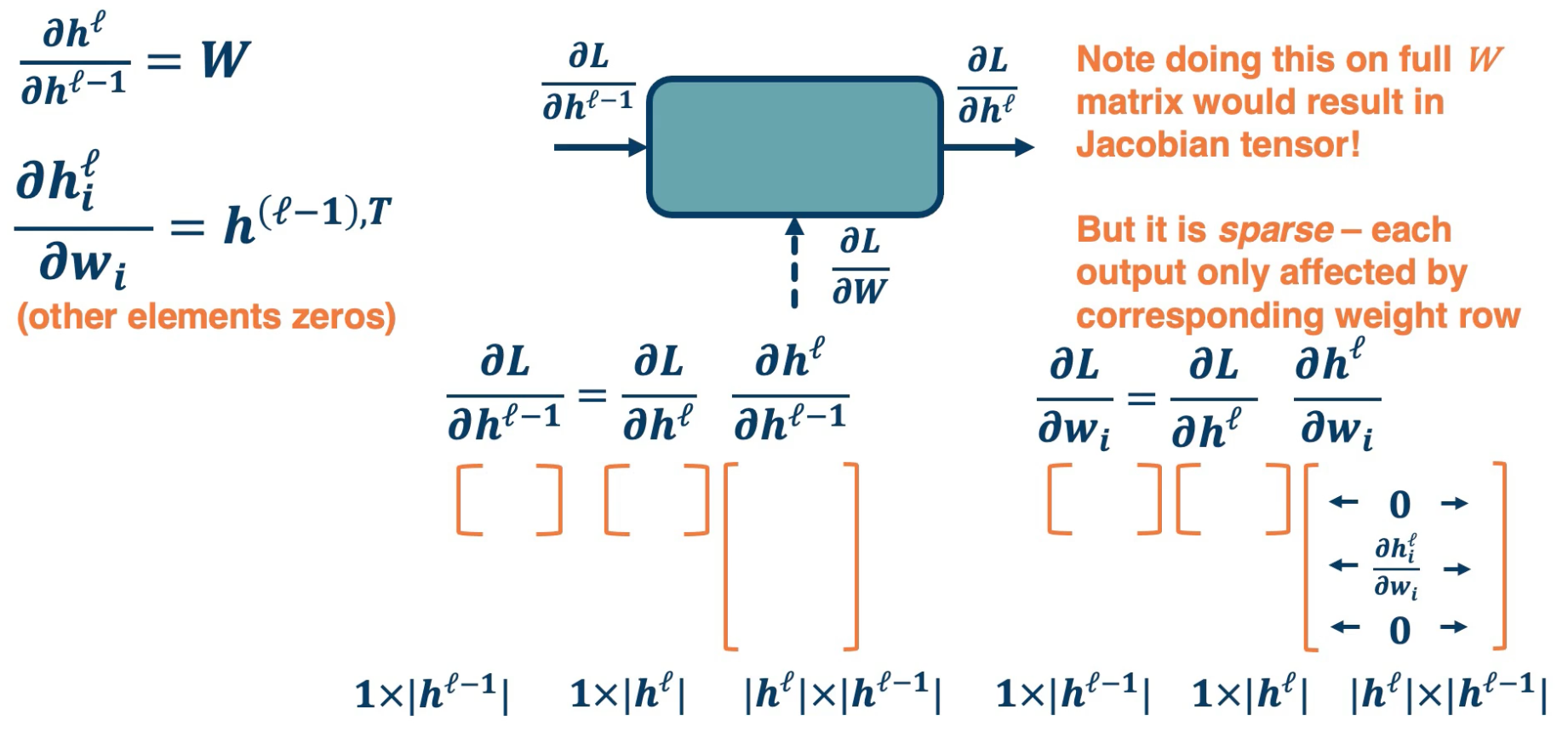
On the left we have the local gradients the partial derivative of the output with respect to the input, which is just $w$ for linear layer. The partial derivative of the output with respect to one particular row in our $w$ matrix, which is equal to the output vector transposed. This is not actually what we need though, what we want is the partial derivative of the loss with respect to our input. We can use chain rule to compute this.
This is equal to the partial derivative of the loss with respect to our output times the partial derivative of the output with respect to our input. This is what we get when we look at the particular sizes of these matrices and vector. The input vector $h^{\ell -1}$ is a column vector. So according to our convention, the partial derivative of a scalar the loss with respect to this column vector is a row vector of size one by the input dimensionality. This is equal to the partial derivative of the loss with respect to our output vector, which also ahs a size of row vector one by our output dimensionality.
We then have the partial derivative of our output with respect to our input. This is a partial derivative of a vector with respect to another vector and so the resulting Jacobian is a matrix whose size is our output dimensionality by the input dimensionality. If you notice the size is all worked out and everything can be reduced into a series of vector to matrix or eventually matrix to matrix multiplications and this can be computed efficiently.
In order to compute our partial derivative of the loss with respect to our weight matrix, we actually boil it down to a particular weight vector rather than doing the whole matrix itself. What we have is the partial derivative of the loss with respect to a particular row in the weight matrix. The row is $w_i$ which according to the last slide is a column vector. And so the resulting size, again, to our convention, is one by the input dimensionality, which is a row vector. This is equal to the chain rule, which is the partial derivative of the loss with respect to our output vector, whose size is again a row vector one by the output dimensionality.
We have the partial derivative of our output with respect to a particular row in the weight matrix. This is a Jacobian matrix but what is interesting is that it has a sparse structure. That is we are looking at a particular row of $w$ which actually affects a particular output node in the output vector. That is, a particular output node $h_i$, because all the other weight rows do not actually affect this particular node, output node $h_i$, all the Jacobians are actually zero expect for that particular row which is equal to the partial derivative of $h^\ell$ with respect to $w_i$.
If we did the partial derivative of the output which is a vector with respect to the entire $w$ matrix, you will have a partial derivative of a vector with respect to a matrix and that is a tensor. We wish to avoid that complexity. It is interesting to note that there is this sparse structure inside the partial derivative of the output with respect to each row in the weight matrix.
Other Functions
As previously mentioned, we can employ any differentiable (or piecewise differentiable function). A common choice is the Rectified Linear Unit (ReLU).
- The ReLU provides non-linearity but better gradient flow than sigmoid so it is preferable over the sigmoid.
- It is also performed element wise. So the function is $h^{\ell} = max(0, h^{\ell-1})$.
- This is not quite differentiable, because there is a discontinuity, but it turns out that there are sub gradients here. We can essentially just take the gradient as being if it is to the left, then zero. If it is exactly to the right, then one. If it is exactly zero, then we can just choose either left or right.
-
How many parameters for this layer?
- The answer is none! It is just taking a max operation and so there are no parameters here.
Now, lets take a look at the Jacobians of gradients for this layer.
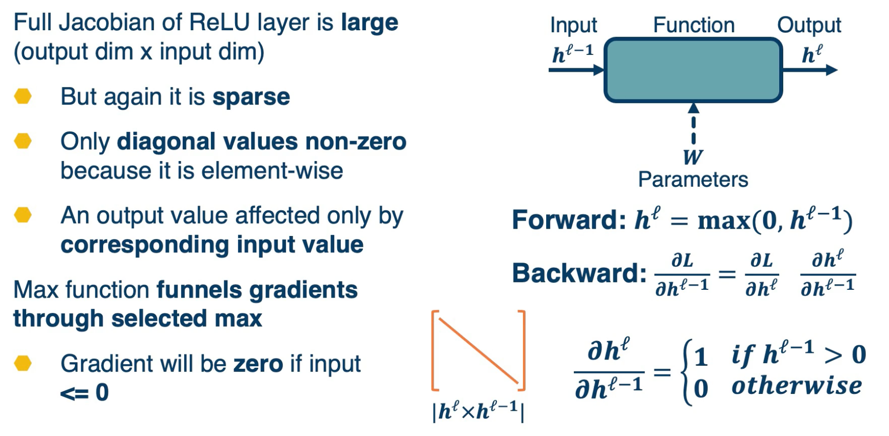
The forward pass is just $max(0,h^{\ell-1})$.
The backward pass can be computed using the chain rule. But if you remember, the max function funnels gradients through the selected max. So the gradient will be zero if the output is $\leq 0$. You can view this as if it is picking the zero part as the maximum then it is not going to funnel the gradients at all, it will have zero gradients.
The full Jacobian of the ReLU is actually large. Its input dimensionality by output dimensionality and actually both dimensionality are the same. However,
- It is sparse
- Only diagonal values non-zero because it is element-wise.
Max Function funnels gradient through selected max
- Gradient will be zero if input $\leq 0$
- This is because an output value is affected only by the corresponding input values. Intuitively, you can think of this as a particular input dimensionality, and $h^{\ell-1}$ only affects the same dimension of the output. It does not affect any of the other ones. And so the non-diagonal entires will all be 0. In other words, changing the particular input dimensionality will have no effect on those outputs. So this is going to be the final Jacobian.
Lesson 3: Optimization of Deep Neural Networks
Readings
Optimization of Deep Neural Networks Overview
A network with two or more hidden layers is often considered a deep model.
Now depth is important for various reasons.
- Structure the model to represent an inherently compositional world.
- Theoretical evidence that it leads to parameter efficiency.
- Gentle dimensionality reduction (if done right)
The world is compositional, we have characters and words and paragraphs and documents in NLP. Or we have object shapes and object parts and scenes in computer vision. So the better that your model reflects this nature or structure in the world, the easier it will be to learn. In other words, you will require less data to learn this function. There are some theoretical evidence that leads to parameter efficiency. For example, there are some functions where if you learn them using a two layered neural network, you will need exponentially more nodes to learn this function than if you just had a three layered neural network. That is, adding depth gives you some parameter efficiency. And as we know in machine learning, dimensionality reduction is crucial. We often start with very high dimensional data such as images or text and what we want to do is gently reduce this dimensionality in order to slowly pick out more and more abstract capable features that are more discriminative for our target classes.
There are still many design decisions that must be made (and this can make or break your model):
- Architecture.
- Often makes learning much easier and need less labeled data``
- Data Considerations
- In ML we know normalization is important.
- Training and Optimization
- Starting with millions or parameters, and we want to start some smart Initialization.
- Machine Learning Considerations.
- Bias vs variance, over fitting etc. We usually have more parameters than data.
We must design the neural network architecture:
- What modules (layers) should we use?
- For example in CV we want different layers compared to NLP.
- In reality alot of these layers are shared across many applications.
- Yet there are still specialized transformations specific to tasks, such as geometric transformation for CV.
- How should they be connected together?
- How the gradient should flow backwards and some can bottle neck the gradient flow?
- Can we use our domain knowledge to add architectural biases?
Lets take a look at some example architectures:
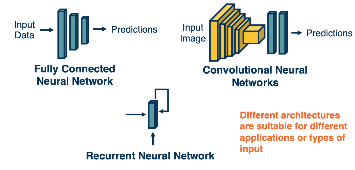
-
Fully Connected Neural Network
- Take an input such as an image, convert it to a vector and feed it through a series of linear and nonlinear transformation. There are hidden layers in the middle and these hidden layers are expected to extract more and more abstract features from high dimensional raw input data. We often reduce their dimensionality or size as we get deeper into the network. At the end, we have a layer that represents our class scores. We have a node that outputs a score for each class and then we combine these to produce probabilities to make our prediction. This architecture is not well suited for several things. For example, images have a lot of input pixels, lets say a million pixels and the number of parameters is equal to the number of input times the number of outputs for a particular layer. IF you think about it, we are not really leveraging the spatial structure in the images. And so they are better suited architectures called convolution neural networks.
-
Convolution neural network
- Rather than tie each node into all pixels in the input, these will reflect only feature extractors for small local windows in the image, that is, will stride a local window across the entire image and each local window will have features extracted from it, such as little shapes, corners or circles or object parts such as eyes or car wheels. We will keep doing this such that at the end we will have features that represent where object parts or entire objects are located in the image. These will be fed to fully connected layers as classifiers.
-
Recurrent Neural Network
- Another downside of fully connected layers is that they represent very fixed size inputs. And so for text where we do not know how many words we will have in a paragraph will actually build a dynamic neural network. We will have a layer for each word in the paragraph and the output of this layer will be dependent on both the input from previous layer that is the vector representing the sentence thus far and the new input that is the new word.
The key point is different architecture are suitable for different applications or different types of input data and it is not always clear what architecture to apply. For example CNN were first developed for images but applied actually to sentences as well. Same for RNN but better architecture came along called transformers.
Similar to traditional machine learning, and actually even more so in deep learning, data is key. So the first step in ML or DL is to really understand your data and go through it. There is also a bunch of design considerations, for example:
- How do we pre-process the raw high dimensional data?
- Should we normalize it?
- Can we augment our data by adding noise or other perturbations?
Even given a good neural network architecture, we need a good optimization algorithm to find good weights.
- What optimizer should we use?
- We talked about gradient descent, but really a specific form of gradient descent which is steepest gradient descent. If we take the negative of the gradient and multiply it by a learning rate, we are taking the direction that is the steepest direction towards the minimum.
- However, there are different optimizers make different weight updates depending on the gradients.
- They still depend on gradients but they might depend on them differently.
- How should we intialize the weights?
- If you start very close to a local minima, getting close to it is not hard and maybe you do not need a great optimizer, just an okay one will be good enough.
- However if your initialization is poorly behaved, then your learning will be much more difficult and you need a much better optimizer.
- What regularizers should we use?
- What loss function is appropriate?
- Talked about cross entropy, RMSE, but there are lots of other things we can apply. We can even design specific loss functions for specific problem.
The practice of machine learning is complex. For your particular application you have to trade off all of the considerations together.
- Trade off between model capacity (measured by number of parameters) and amount of data.
- This is not a straight forward task and there is not really a lot of theory that tells you exactly what to do here.
- Unfortunately in neural network you often want a high capacity, this is why neural networks have failed in the pass because researchers only tried low capacity networks.
- Adding appropriate biases based on domain knowledge will make learning faster.
- However this can be a double edge word if your domain knowledge turns out to be incorrect.
Architectural Considerations
In this lesson, we will talk about architectural consideration and specifically, what types of non-linearities you should use.
Determining what modules to use, and how to connect them is part of the architectural design
- Should be guided by the type of data used and its characteristics and your application.
- Understanding your data is always the first step!
- Fortunately, there are lots of data types (modalities) already have good architectures that researchers that have already look at.
- Start with what others have discovered is one of the key ways that you can speed up the deep learning process.
-
The flow of gradients is one of the key principles to use when analyzing layers.
- Backpropagation lives or dies by gradient.
- You can have modules that accidentally bottleneck or stop gradient flow thats effective.
Deep neural networks consist of a sequence/combination of linear and non linear layers.
- Combination of only linear layers has the same representational power as one linear layer.
- This is is because you can just take the $W$ matrix and multiply them together.
-
Non-linear layers are crucial.
- They increase the representational power of DNN and they allow you to perform complex transformations of the data.
- This complexity comes at a cost, the gradient flow across non-linearities heavily depends on their shape.
There are several aspects that we can analyze to see how a particular non-linearity will behave. We can take a look at:
- Min/Max
- Correspondence between input and output statistics.
-
Gradients
- At initialization
- For example, it depends on what the non-linearity looks like and specifically the derivative look like. In order to understand that when we have small weight values, how we initialize these weights, what will the actual gradients look like? Will it vanish? or explode?
- At extremes
- For example some gradients flatten out to be 0 at the end when you have large values fed into it. Others stay linear at all portions of the function.
- At initialization
- Computational complexity
- Some piece-wise linear functions are super fast to compute because they’re just max functions. Others require computing exponentials or division, and so those might be more complex.
Lets look at some examples of non-linearity functions and their behavior:
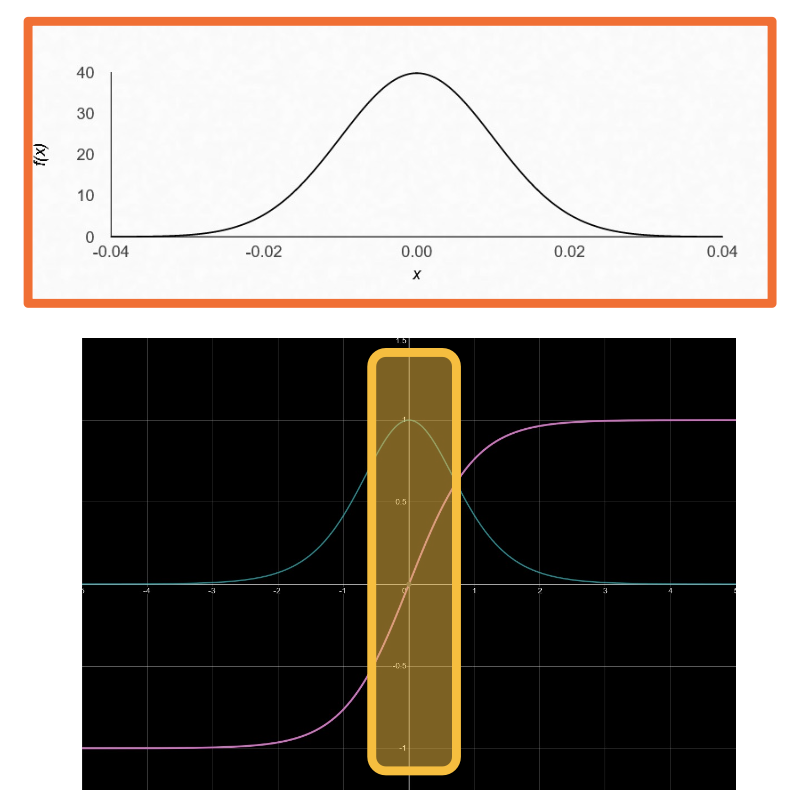
sigmoid
-
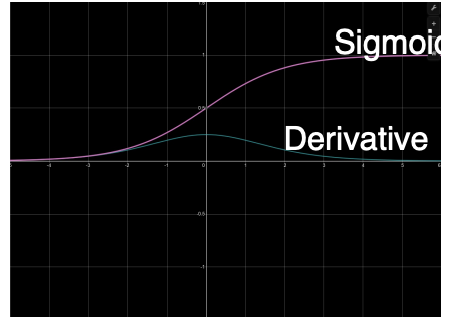
Sigmoid
- Min 0, Max 1
- Output is always positive
- Saturates at both ends
- gradients
- Vanishes at both end (converging to 0)
- Always positive
- Computation: exponential term
When we have an upstream gradient, and then we multiply that by the local gradient, the gradient of our function. Now if we received very high values as input, then our gradients are going to be very small, vanishingly small. This will cause issue for two reasons.
First, this partial derivative of the loss with respect to the weights, which is what we use to update the weight using gradient descent will become a very small number because you’re multiplying a very small gradient by the upstream gradient. The worse issue is that we are also passing back the gradient, and the change in loss with respect to our inputs is what we pass back, and that is the upstream gradient for the previous module. If we pass back a small learning gradient, then the previous module will also have a lower learning rate essentially, and it won’t learn very much. This vanishing gradient problem is not only one that is a problem for this module, but it accumulates as it goes backward.
Note that the fact that it is also minimum of 0 and maximum of 1 means that it can also explode going forward. So if we pass a higher value, meaning that we always pass positive values, so we keep passing higher values, and those higher values will then be fed into the next non-linearity potentially and become even larger if its the same non-linearity.
So, there are alot of issues with the sigmoid function, both going forward and backward.
TanH
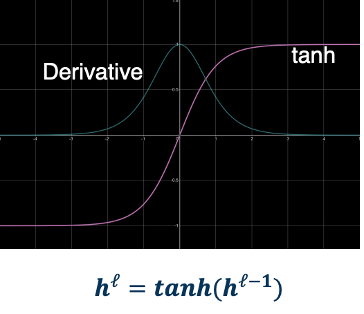
-
tanh
- Min -1, Max 1
- Centered
- Saturates at both ends
- gradients
- Vanishes at both end
- Always positive
- Still somewhat Computationally heavily
- Min -1, Max 1
Same shape as sigmoid but -1 to 1 which means it is a balanced or centered function. It can also provide negative outputs, meaning it can flip the sign of different features. However it is still saturated at both ends, so it has the same issue as sigmoid.
ReLU
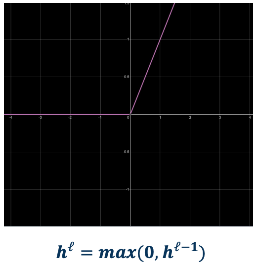
-
ReLU
- Min 0, Max infinity
- Output is always positive
- No saturation on positive end
- gradients
- 0 if $x \leq 0$ (dead ReLU)
- Constant otherwise (does not vanish)
- cheap to compute (max)
The gradient flow is much better as there is no saturation on the positive end. However, if it ls less than 0, the gradients are again 0 and this is an issue and have the issue what is called a dead ReLU which is a ReLU that has inputs coming to it with negative values and then it will not really learn anything because its gradients are 0. However notice that it is never the fact that there is only one ReLU tied to any input. You have inputs tied to many ReLUs and so those other ReLUs can maybe push the values of the inputs to become more positive.
On the positive side of the curve, it is a constant gradient and so it does not vanish, which is a good thing.
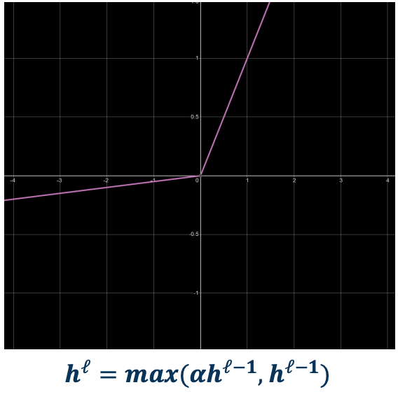
Leaky ReLU
-
leaky ReLU
- Min -infinity, Max infinity
- Learnable parameter!
- No saturation
- gradients
- No Dead neuron
- cheap to compute (max)
Leaky ReLU tries to address the dead ReLU problem. It is the same thing on the positive side but on the negative side it has a slight slope. You can even add a parameter to learn the slope.
Whenever you want the neural network to have some flexibility to learn something beyond what you are actually programming in terms of the functions, then you should parameterize those functions so that it can have a little bit of flex and can learn those parameters.
One thing you might notice that this is not a differentiable function, but it turns out to be actually ok. We can have what are called subgradient, which means as long as there is a finite number of components to the function that have gradients that we can compute, its fine. For example in this function if $f$ is $0$ we can choose either side in terms of computing the gradient.
Conclusion
Unfortunately, no one activation function is best for all applications.
-
ReLU is most common starting point
- sometimes leaky ReLU can make a big difference
- Sigmoid is typically avoided unless clamping to values from $[0,1]$ is needed.
Initialization
In this lesson, we will talk about intelligent initialization of the parameters for DNN. This is important because if you initialize the weights to values that are degenerate in some way, for example for very close to bad local minima or lead to poor gradient flow during backward pass, then learning is not going to be effective.
The parameters of our model must be initialized to something.
- initialization is extremely important
- It determines how the statistics of our output given the input behave behave.
- Determines how well Gradients flow in the beginning of training.
- Could limit use of full capacity of the model if done improperly.
- Initialization that is close to a good (local minima) will converge faster and to a better solution.
For example, if you initialize the weights such that the activations tend to statistically be large, and these large activations are fed to non-linearities such as the tnaH function, then you will start in the saturation range of these non-linearities which causes ineffective learning (or worse, none).
However, if you initialize your weights such that the inputs to these activations are actually very small values, you will be in the linear regime or close to it of these non-linearities in the space where the inputs are close to zero. Then you will have strong gradient to work with.
Poor initialization
Lets take a look at an example of bad initialization.
For example, initializing values to a constant value leads to a degenerate solution.
- What happens to the weight updates?
- Each node has the same input from previous layers so gradients will be the same
- As a result, all weights will be updated to the same exact values.
These are bad initialization unless for some reason you want the weight to move together. We will see applications of this later on.
Normal Initialization
A common approach is to initialize your model is using small normally distributed random numbers.
- E.g $N(\mu, \sigma), \mu = 0, \sigma = 0.01$
- Small weights are preferred since no feature/input has prior importance.
- Keeps the model within the linear region of most activation functions.
This is a very safe and reasonable approach that is still widely used.
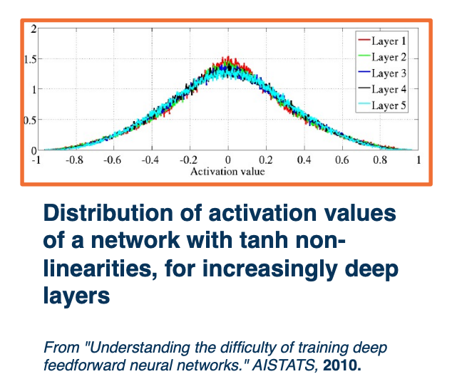
Deeper networks (with many layers) are more sensitive to initialization
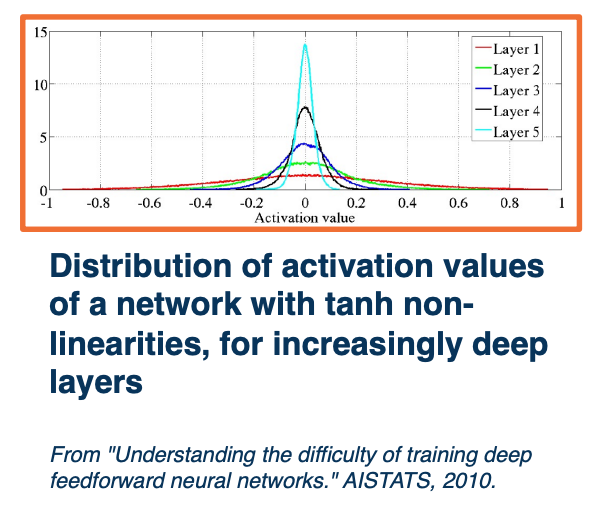 As seen, layer 5 has activations has very small standard deviation but layer one has a larger standard deviation and a much smaller set of values
- With a deep network, activations (outputs of nodes) get smaller
- Standard deviation reduces significantly
- Leads to small updates - smaller values multiplied by upstream gradients
- Larger initial values lead to Saturation
Recall, if your non-linearity is tanh or sigmoid, then you will have gradients that are very small at the end and we don’t want either too small or too large of values. We do not want this distribution to really change across the depth of the neural network. What we want to do is to finally balance this. Unfortunately, balancing this is not easy and it depends on specific modules you pick.
Xavier Initialization
Ideally, we’d like to maintain the variance at the output to be similar to that of input!
Specifically, we do not want the variance to shrink as we get deeper into the network. There is no reason to start using a smaller variation or range of values in our activation outputs, which is what that means. We also do not want to increase the variance, we just want to maintain the variance to be the same at initialization.
For example, this shows the activation functions across a range of different layers in a deep neural network using the Xavier initialization. You can see that unlike the previous plot across all the different layers, the distribution is very similar which is what we want. The derivation of the actual weight initialization so this condition is omitted, but it actually leads to a very simple initialization.
What we do is we sample from a uniform distribution between a negative positive value.
\[U\bigg(-\frac{\sqrt{6}}{\sqrt{n_j+n_{j+1}}}, + \frac{\sqrt{6}}{\sqrt{n_j+n_{j+1}}}\bigg)\]- Where $n_j$ is fan-in (number of input nodes)
- and $n_{j+1}$ is fan-out (number of output nodes).
This makes sense intuitively, because we are dividing by these values. For example if a particular node has a large number of inputs, then we probably want to tune down the weights, because we are summing up the weighted summation of the inputs. Conversely, if a node has very few inputs, then we may want to increase the weight.
(Simpler) Xavier and Xavier2 Initialization
In practice, simpler versions perform empirically well:
\[N(0,1) * \sqrt{\frac{1}{n_j}}\]- This analysis holds for tanh or similar activations
- Similar analysis for ReLU activations leads to:
Typically for each activation function you like to try, you need to do a similar analysis, either theoretical or empirical. In the case of ReLU, it is very similar to Xavier and infact it is called Xavier2 and more details can be found in the paper.
In summary, Initialization matters!
- Determines the activation (output) statistics, and therefore Gradient statistics
- If the gradients are *small, no learning will occur and no improvement is possible.
- Important to reason about output/gradient statistics and analyze them for new layers and architectures.
Preprocessing, Normalization, and Augmentation
In deep learning, data drives learning of features and classifier.
- Its characteristics are therefore extremely important.
- Always understand your data
- Relationship between output statistics, layers such as non-linearities, and gradients is important.
Just like initialization, normalization can improve gradient flow and learning.
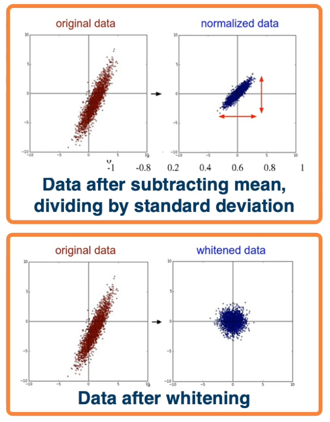
Typically, normalization methods apply:
- Subtract mean, divide by standard deviation (most common)
- This can be done per dimensional
- Whitening, e.g through PCA (not common, and often not necessary)
We can try to come up with a layer that c an normalize the data across a network.
Given: A mini-batch of data $[\textbf{B} \times \textbf{D}]$ where $\textbf{B}$ is batch size,
Compute mean and variance for each dimension $d$:
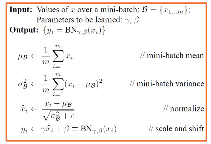
Note that $\hat{x_i}$ denominator has a small $\varepsilon$ so that it does not blow up incase the variance is small. This part does not involve new parameters.
- We can give the model flexibility through learnable parameters $\gamma$ (scale) and $\beta$ (shift)
- Network can learn to not normalize if necessary.
- This layer is called a Batch Normalization (BN) layer.
There are some complexities of BN:
During training, we compute mean and variance over your mini batch each iteration. So you are normalizing by a different amount each time because your number of samples might be small in each batch compared to large amount of data you have. So there is some noise in the estimation of the means and variances.
However during inference, stored mean/variances calculated across the entire training set are used. So this means:
Sufficient batch sizes must be used to get stable per-batch estimates during training
- This is especially an issue when using multi-GPU or multi-machine training
- Use
torch.nn.SyncBatchNormto estimate batch statistics in these settings.
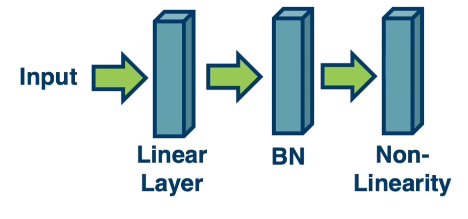
Normalization especially important before non-linearities.
Very low/high values (un normalized/imbalanced data) can cause saturation.
There are many variations of batch normalization, we will see some in CNN later.
Optimizers
So far we only talked about SGD, namely steepest descent which is only one way to update the weights. We will talk about more sophisticated methods.
Deep learning invovles complex, compositional, non-linear functions. This means that the loss landscape is extremely non-convex as a result. There is little direct theory and a lot of intuition/rules of thumbs instead. Some insight can be gained via theory for simpler cases (such as convex settings)
It used to be thought that Existence of local minima is the main issue in optimization. There are other more impactful issues:
- Noisy gradient estimates
- Could be because we take mini batches of data
- Saddle points
- Ill-conditioned loss surface.
Noisy gradients
In practice, we use a subset of the data at each iteration to calculate the loss (and gradients).
This is actually an unbiased estimator, meaning that the expectation is equal to the true non-stochastic full batch value (value of the gradients if we just calculate them on our entire training set). However that is only on expectation, in reality we will have high variance.
This results in noisy steps in gradient descent.
Loss surface Geometry
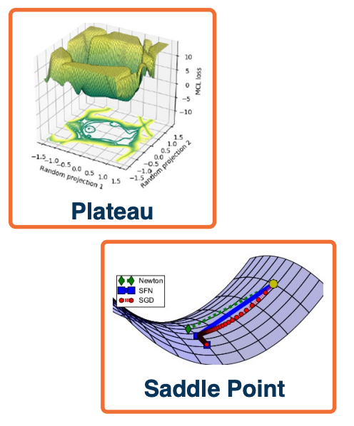
Several loss surface geometries are difficult for optimization.
Several types of minima: Local minima, plateaus, saddle points
Saddle points are those where the gradient of orthogonal directions are zero but they disagree (its min for one, max for another). In other words, its a minimum for one direction but a maximum for another.
Saddle points are much more common in these high dimensional optimization problems that are induced by deep learning.
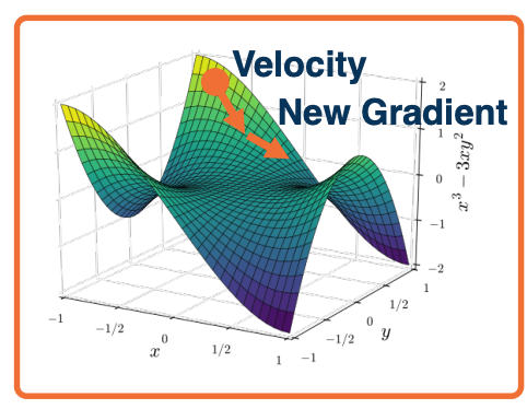
Adding momentum
- Gradient descent takes a step in the steepest direction (negative gradient) $w_i = w_{i-1} - \alpha \frac{\partial L}{\partial w_i}$ doesn’t necessarily behave very well in these saddle point regions. They will either get stuck or learn very slowly.
- Intuitive idea*: Imagine a ball rolling down loss surface, and use momentum to pass flat surfaces.
Rather than just update the negative gradient, we first calculate a velocity term, where $v_0 = 0$ and $\beta$ starts at $0.99$. So Beta is almost like decaying your velocity and adding your current gradient.
Your weights $w_i$ will then be updated by the velocity term and not by the local gradient that you have now. This can pop you out of local plateaus or saddle points as long as gradients remains in the same direction.
\[\begin{aligned} v_i &= \beta v_{i-1} + \frac{\partial L}{\partial w_{i-1}} & \text{(Update Velocity)}\\ w_i &= w_{i-1} - \alpha v_i & \text{(Update Weights)} \end{aligned}\]This is a generalization of SGD where $\beta = 0$.
Accelerated Descent methods
Velocity term is an exponential moving average of the gradient, notice the recurrent relationship:
\[\begin{aligned} v_i &= \beta v_{i-1} + \frac{\partial L}{\partial w_{i-1}}\\ &= \beta \bigg( \beta v_{i-2} + \frac{\partial L}{\partial w_{i-2}} \bigg) + \frac{\partial L}{\partial w_{i-1}}\\ &= \beta^2v_{i-2} + \beta \frac{\partial L}{\partial w_{i-2}} + \frac{\partial L}{\partial w_{i-1}} \end{aligned}\]There is a general class of accelerated gradient methods, with some theoretical analysis (under certain assumptions)
Equivalent Momentum Update
Another form can be re-written as (where $v_0 = 0$):
\[\begin{aligned} v_i &= \beta v_{i-1} - \alpha \frac{\partial L}{\partial w_{i-1}} & \text{(Update Velocity)}\\ w_i &= w_{i-1} - \alpha v_i & \text{(Update Weights)} \end{aligned}\]Nesterov Momentum
Rather than combining velocity with current gradient, go along velocity first and then calculate gradient at new point since we know velocity is probably a reasonable direction
Extra reference for this topic
Hessian and loss curvature
- Various mathematical ways to characterize the loss landscape
- The jacobian (first order) only tells you the steepest direction but leads to some limitations such as what step size to take which is why we have things like learning rate.
- The hessian gives us information about the curvature of the loss surface
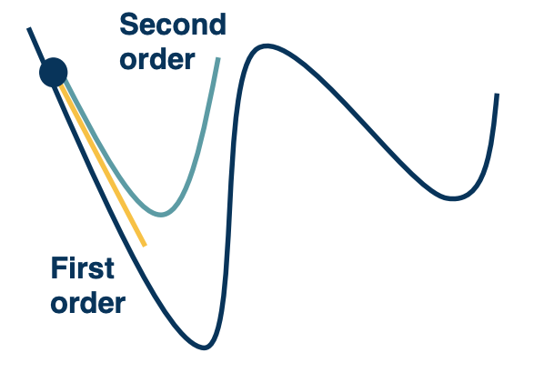
(Remember where the second derivative tells you if its the maximum or minimum?)
We can use tricks like Taylor series expansion, we can actually perform a quadratic approximation of the loss surface around the current weights in the weight space. The advantage of this is that we can just jump directly to the minima of that approximation.
In practice these methods are not used very frequently thats because computing the hessian is expensive but actually things like momentum actually approximate this to some degree.
Condition number
Condition number is the ratio of the largest and smallest eigenvalue of the Hessian matrix.
- Tells us how different the curvature is along different dimensions.
If this condition number is high, that means that different directions actually point to very different curvatures. SGD will make big steps in some dimensions and small steps in other dimensions. This is a problem, because what you will have is what you see below:
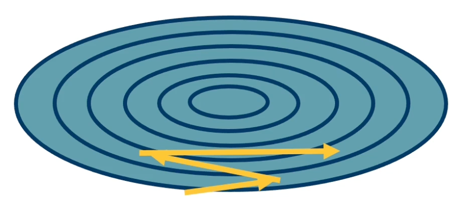
You will have large jumps in certain directions because the curvature is very high and that means that along the directions that the curvature is not so high, you actually will not get very effective learning.
Second-order optimization methods divide steps by curvature, but expensive to compute. So we will look at alternative methods that are much more efficient.
Per parameter learning rate
Have a dynamic learning rate for each weight, there are several flavors of optimization algorthims:
- RMSProp
- Adagrad
- Adam
- …
SGD can achieve similar results in many cases but with much more tuning. Again certain methods works well under certain conditions or may not generalize as well as SGD plus momentum. However, SGD with momentum takes a lot of tuning to get it right.
For most applications DL do pretty well without requiring tuning so that is why algorthims such as Adam are typically preferred to start with.
Adagrad
Idea: Use gradient statistics to reduce learning rate across iterations. We are going to have a gradient accumulator $G_i$ which takes the previous accumulation plus our gradients squared.
Now, when we perform a weight update, unlike doing the normal negative alpha times the gradient, which we do in the steepest gradient descent, we are going to divide the learning rate by the square root of $G_i$ plus some epsilon. What we are effectively doing is for each weight, basically toggling the learning rate down based on how much gradient or how strong the gradients are for that weight. And if you have some weights that have very strong gradients where very high curvature probably along that dimension, then we are going to tone down the learning rate.
Where as if there are other weights that have smaller grading, then we are going have a smaller value in the denominator and then a higher effective learning rate.
\[\begin{aligned} G_i &= G_{i-1} + \bigg( \frac{\partial L}{\partial w_{i-1}} \bigg)^2 \\ w_i &= w_{i-1} - \frac{\alpha}{\sqrt{G_i + \varepsilon}} \frac{\partial L}{\partial w_{i-1}} \end{aligned}\]- Denominator: Sum up gradients across iterations
- Directions with high curvature will have higher gradients and learning rate will reduce.
However there is one problem with this, as gradients are accumulated $G_i$ gets bigger and bigger, the learning rate $\frac{\alpha}{\sqrt{G_i + \varepsilon}} $ will go to zero.
RMSProp
Solution: Keep a moving average of the squared gradients! This does not saturate the learning rate - the gradient does not go to zero as the gradients $G_i$ accumulates higher and higher.
\[\begin{aligned} G_i &= \beta G_{i-1} + (1-\beta) \bigg( \frac{\partial L}{\partial w_{i-1}} \bigg)^2 \\ w_i &= w_{i-1} - \frac{\alpha}{\sqrt{G_i + \varepsilon}} \frac{\partial L}{\partial w_{i-1}} \end{aligned}\]Adam
Combine ideas From RMSProp and Adagrad. Maintains both first and second moment statistics for gradients.
\[\begin{aligned} v_i &= \beta_1 v_{i-1} + (1-\beta_1) \bigg( \frac{\partial L}{\partial w_{i-1}}\bigg)\\ G_i &= \beta_2 G_{i-1} + (1-\beta_2)\bigg( \frac{\partial L}{\partial w_{i-1}} \bigg)^2 \\ w_i &= w_{i-1} - \frac{\alpha v_i}{\sqrt{G_i + \varepsilon}} \end{aligned}\]The initial values for $v_i$ and $G_i$ typically start out as 0. So these are going to be pretty small values and you are going to update them using the current gradient at whatever initialization you start out with. Then you will essentially have this tiny gradient and these values will be very small. So you are multiplying alpha by some arbitrary small value and dividing by some arbitrary small value. Also, the $G_i$ is a squared term so it depends on what the gradient will be. In some cases it could be much higher or in some cases if its less than 1,then it will be lower.
In order to address this instability, we are going to do some time varying smoothing of these values such that in the beginning we will try to perform less biased estimates and then over time, we will just converge to these actual values that are shown here.
So, this is the final Adam algorithm with new terms $\hat{v} \text{ and } \hat{G}$.The purpose of these is really to stabilize the initial values. The solution will be a time-varying bias correction. Typically $\beta_1 = 0.9, \beta_2 = 0.999$.
\[\begin{aligned} v_i &= \beta_1 v_{i-1} + (1-\beta_1) \bigg( \frac{\partial L}{\partial w_{i-1}}\bigg)\\ G_i &= \beta_2 G_{i-1} + (1-\beta_2)\bigg( \frac{\partial L}{\partial w_{i-1}} \bigg)^2 \\ \hat{v_i} &= \frac{v_i}{1-\beta_1^t}\\ \hat{G_i} &= \frac{G_i}{1-\beta_1^t}\\ w_i &= w_{i-1} - \frac{\alpha \hat{v}_i}{\sqrt{\hat{G}_i + \varepsilon}} \end{aligned}\]So $\hat{v}_i$ will be small number divided by (1-0.9 = 0.1) resulting in more reasonable values (and $\hat{G}_i$ larger). As $t$ increases then the denominator will become 1 and $\hat{v}_i$ will take their actual values, similar for $\hat{G}_i$.
One thing to note is that even though Adam changes the learning rate per parameter or weight, and actually still has some learning rate $\alpha$. So its not like you are escaping the fact that you still need to hyper parameter tune the learning rate.
Behavior of Optimizers
Optimizers behave differently depending on landscape. Different behaviors such as overshooting, stagnating etc.
Plain SGD+momentum can generalize better than adaptive methods, but require more tunning.
Learning rate schedules
First order optimization methods have learning rates
Theoretical results rely on annealed learning rate
Several schedules that are typical:
- Graduate student! (lol)
- Step scheduler
- Change the learning rate say divided by 10 every few epochs or n epochs.
- exponential scheduler
- Cosine scheduler
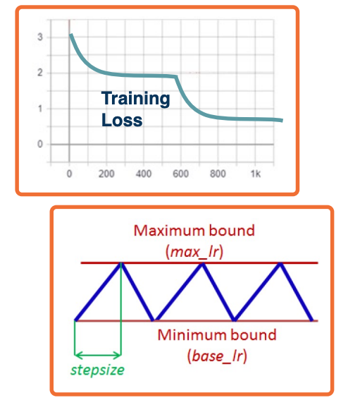
- Continuously reduce and increase the learning rate up again works quite well in practice. You can think of this as popping the model out of that local minima to find maybe a better local minima. Then you can figure out which model gave you the best results and figure out which local minima was the most generalizable to the validation.
Regularization
Many standard regularization methods still apply!
- L1 : $L= \lvert y - Wx_i \lvert ^2 + \lambda \lvert W \lvert $
- L1 encourages sparsity - alot of values close to zero and only a few non zeros
- L2 : $L = \lvert y-Wx_i \lvert^2 + \lambda \lvert W \lvert ^2$
- L2 encourages weights to be small
- Elastic Net: $L = \lvert y - Wx_i \lvert ^2 + \alpha \lvert W \lvert ^2 + \beta \lvert W \lvert$
Dropout
Problem: Neural network can learn to rely strong on a few features that work really well.
- may cause overfitting if not representative of test data
An idea: For each node, keep its output with probability $p$.
So at each node, determine whether to keep the activations from that node or not. If I do not keep it, activations of deactivated nodes are essentially zero. So computing the forward and backward function is not affected by that node.
In practice, it is implemented with a mask calculated each iteration:
During testing, no nodes are dropped (during testing all nodes are used).
However, this presents a problem:
- During training, each node has an expected $p \times \text{fan_in}$ nodes
- During test all nodes are activated.
- Principle: Always try to have similar train and test-time input/output distributions.
- This violates the above principle, how?
Solution: During test time, scale outputs (or equivalently weights) by $p$.
- $W_{test} = pW$
- alternative: Scale by $\frac{1}{p}$ at train time.
- Then during testing time you do not need to do anything else.
Why Dropout works
-
Interpretation 1: The model should not rely too heavily on particular features.
- It it does, it has probability $1-p$ of losing that feature in an iteration.
- During backpropagation, it will update the weights of other features.
- Equalizing the weights across all of the features such that it does not rely too heavily on any specific subsets.
-
Interpretation 2: Training $2^n$ networks
- That is, if you think about the number of masks that you can create, the number of configurations that there are for $n$ node neural network is $2^n$.
- Most are trained with 1 or 2 mini batches of data.
- Essentially having an ensembling effect - you are training many simpler networks (due to drop out) and trying to combine them together at the end.
Data Augmentation
Performs a range of Transformations to the data.
- This essentially “increases“your dataset.
Transformations should not change meaning of the data (or label has to be changed as well)
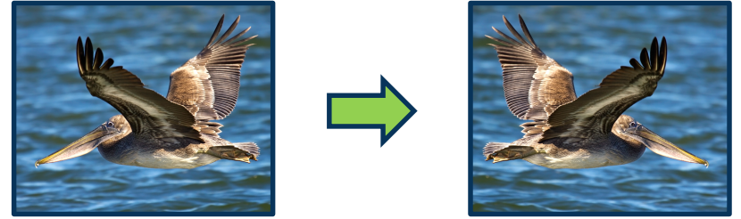
- Flipping:
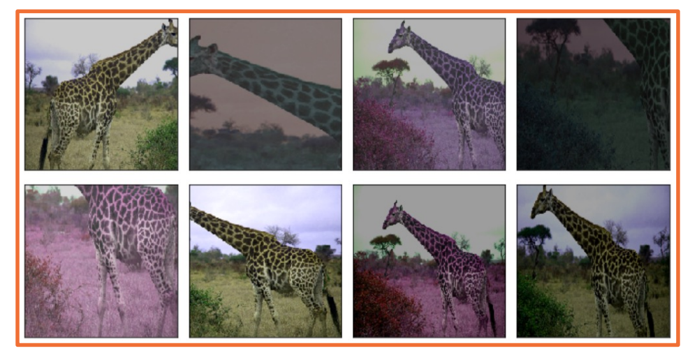
- Random Crop
- Can also do it during testing
- For example, average the probabilities over all of these different crops.
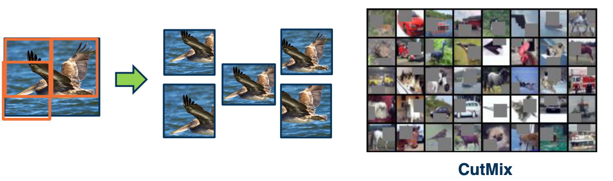
- CutMix
- Cutting and mixing different images together.
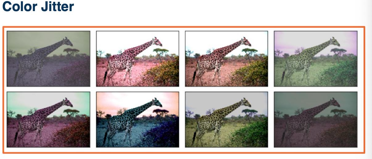
- Color Jitter
- Add or subtract RGB pixels from the image.
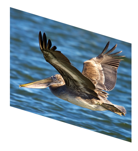
- Generic affine transformation such as Translation, rotation, scale, shear
Can be combined:
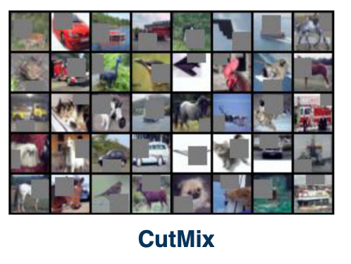
CowMix:
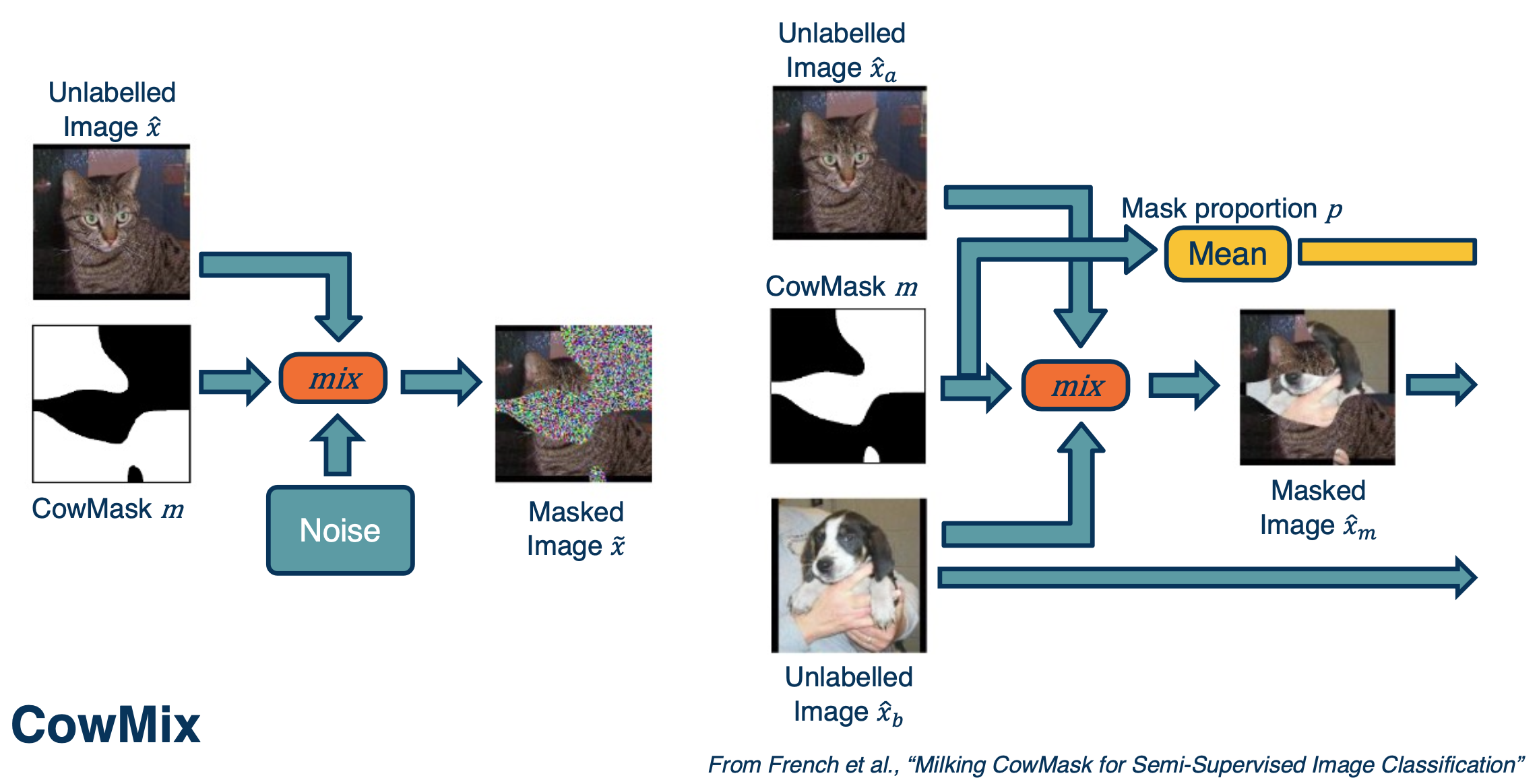
On the left, you are combining an image of a cat with some kind of cow looking pattern in terms of a mask. These masks determine whether to take pixels from the image, which is the cat, or to take pixels from the noise. This forces the neural network to be very robust to things like occlusion.
On the right side you can see a more complicated example. The question is what should the ground truth be over here? You can actually make the ground truth label proportional to how many pixels you took from the cat and dog.
The Process of Training Neural Networks
- Training deep neural networks is more of an art form than science.
- Lots of things matter and they matter together
- The key is to find a magical combination that works and allow it to learn a really good function for your application.
-
Key principle: Monitoring everything to understand what is going on.
- Can print out every gradient, activation and every loss value that happens across your entire optimization.
- Loss and accuracy curves
- Gradient statistics / characteristics
- Other aspects of computation graph
Analyzing what is going on in your particular Deep Learning application always starts with proper methodology.
- Not uncommon even in published papers to get this wrong.
Separate data into: Training, validation, test set
- Do not look at test set performance until you have decided on everything (including hyper parameters)
Use cross-validation to decide on hyper parameters if amount of data is an issue.
Sanity check
Check the bounds of your loss function
- e.g cross entropy ranges from $[0, \infty]$
- Check initial loss at small random weight values
- e.g $-log(p)$ fro cross-entropy where $p=0.5$
Another example: Start without regularization and make sure loss goes up when added
Key principle: Simplify the dataset to make sure your model can properly (over)-fit before applying regularization.
Loss and Not a Number (NaN)
-
Changes in loss indicates speed of learning
- Tiny loss change -> too small of a learning rate
- Loss (and then weights) turn into
Nans-> too high of a learning rate
-
Other bugs can also cause this:
- Divide by zero
- Forgetting the log!
In pytorch, use autograd’s detect anomaly to debug:
1
2
3
4

with autograd.detect_anomaly():
  output = model(input)
  loss = criterion(output, labels)
  loss.backward()
Overfitting
- Classic machine learning signs of under/overfitting still apply
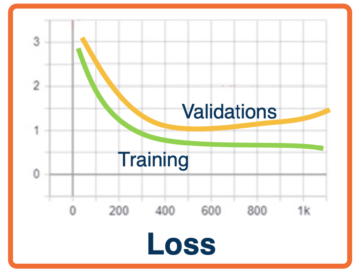
- Over-fitting - validation loss/accuracy starts to get worse after a while
- Under-fitting - validation loss very close to training loss or both are high
- Note, you can have higher training loss!
- Validation loss has no regularization
- Validation loss is typically measured at the end of an epoch. So it may not be surprising if your validation loss is better than your training loss.
Hyper-parameter tuning
Many high-parameters to rune!
- learning rate, weight decay crucial
- Momentum, others more stable
- Always tune hyper parameters, even a good idea will fail untuned.
Start with coarser search:
- E.g learning rate of
0.1, 0.05, 0.003, 0.01, 0.003, 0.001, 0.0005,0.0001 - Perform finer search around good values
Note that hyper-parameters and even module selection are interdependent!
Examples:
- Batch norm and dropout maybe not be needed together and sometimes the combination is worse
- The learning rate should be changed proportionally to batch size - increase the learning rate for larger batch sizes
- One interpretation: Gradients are more reliable/smoother
Relationship between loss and other metrics
Note that we are optimizing a loss function
What we actually care about is typically different metrics that we cannot differentiate
- accuracy
- Precision/Recall
- other specialized metrics
The relationship between the two can be complex!
Simple example: Cross-entropy and accuracy
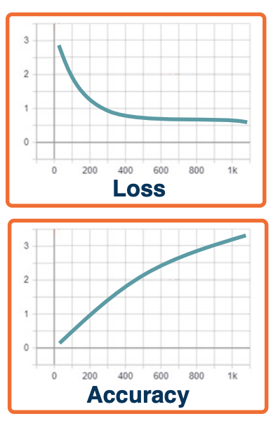
- Example: Cross entropy loss $L=-log(P=y_i \lvert X=x_i)$
- Accuracy is measured based on $argmax_i (P(Y=y_i \lvert X=x_i))$
- Since the correct class only has one to be slightly higher, we can have flat loss curves but increasing accuracy!
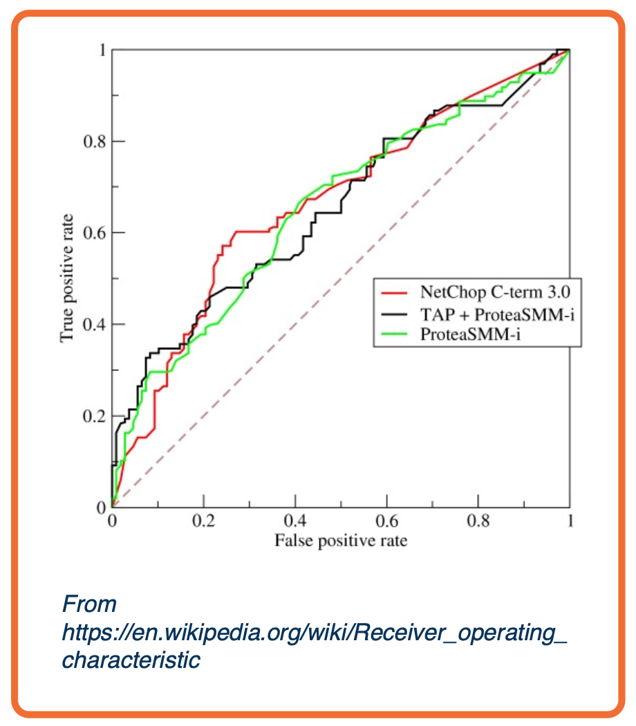
Precision/Recall or ROC curves
-
TPR/FPR curves represent the inherent tradeoff between number of positive predictions and correctness of predictions
- Receiver operating characteristics (ROC) curves similar, plot precision/recall instead.
- Precision/recall curves represent the inherent tradeoff between number of positive predictions and correctness of predictions
Definitions:
- True positive rate: $TPR = \frac{tp}{tp+fn}$
- Also known as recall
- False positive rate: $FPR = \frac{fp}{fp+tn}$
- Accuracy = $\frac{tp+tn}{tp+tn+fp+fn}$
- Precision = $\frac{tp}{tp+fp}$
We can obtain a curve by varying the probability threshold and plot out TPR, FPR to get AUC:
- Area under the curve (AUC) common single number metric to summarize
- Mapping between this and loss is not simple!
Lesson 4: Data Wrangling
Readings
- General preprocessing: Preprocessing for deep learning: from covariance matrix to image whitening
- General preprocessing: cs231n on preprocessing
- Optional: Khetarpal, Khimya, et al. Re-evaluate: Reproducibility in evaluating reinforcement learning algorithms. (2018). See related blog post
Data Cleaning for Machine Learning
- Clean
- Transforma
- Pre-Process
Missing Data Mechanisms
-
Missing completely at random: likelihood of any data observation to be missing at random
- if someone forgot to fill out a depression survey answer, that would be missing completely at random.
-
Missing at random: likelihood of any data observation to be missing depends on observed data features
- Males tend to not fill up a depression survey, so this would be missing at random.
-
Missing not at random: likelihood of any data observation to be missing depends on unobserved outcome.
- Someone did not fill up as a direct causation of their depression
Cleaning data - Ways to fill up missing data:
- Discard missing rows
- loses information
- Imputation
- Numerical Data
- Mean, mode, most frequent, zero, constant
- Categorical Data
- Hot-deck imputation, K-nearest neighbors, deep learning embeddings
- Numerical Data
Transforming
- Image
- Color conversation
- Maybe from RGB to grayscale
- Color conversation
- Text
- Index:
- (Apple, Orange, Pear) -> (01,2)
- Bag of Words
- Term-frequency times inverse document frequency (TF-IDF)
- L1 normalization of the rows of a matrix
- Embedding
- Index:
Pre-preprocessing
- Normalize / Zero-center
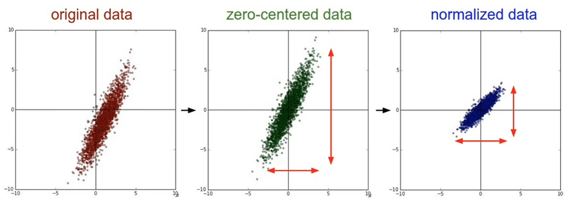
Case Study - depth estimation
For depth estimation, we are predicting at every pixel in the image the distance from the camera.
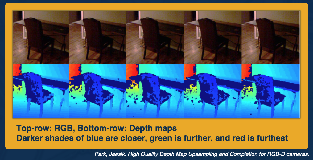
Usually, depth sensors predict very noisy data. You can see the holes in the depth images in the second row here. So the first step we need to do is clean these holes, clean the data.
There are many ways to fill in the missing depth values (black pixels in depth map)
- Nearest Neighbor (naive)
- Colorization (NYU Depth V2)
- Uses inpainting to find the missing results
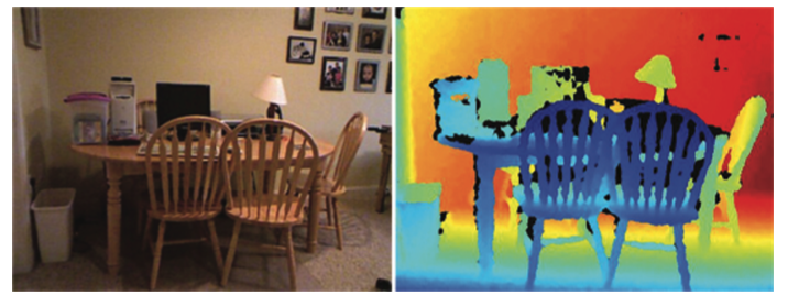
This is how the depth map looks like after we hae filled in all the missing values:
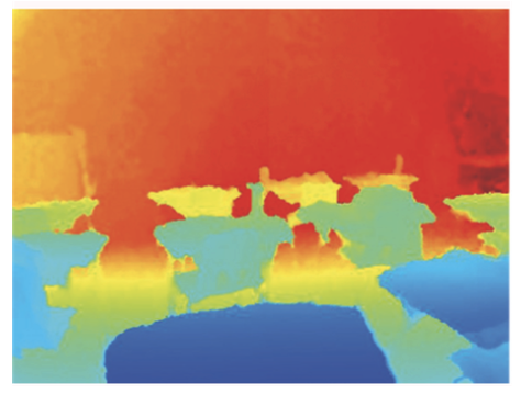
The next step is to transform our data. Learning rich features from RGB-D images for object detection and segmentation found that instead of using a single channel depth map, they see improved performance by using 3 channels as the input.
Transform the 1-channel depth map into 3 channels:
- Horizontal disparity
- Height above ground
- Angle with gravity
The final step is pre processing, for depth estimation, inverse depth helps to:
- improve numerical stability
- Gaussian error distribution
For example, see in the chart below without normalization, training quickly collapses and our mean depth goes to zero. However with normalization we are able to train for long periods of time without our depth collapsing to zero.
Managing Bias
There are many mathematical definitions of fairness in machine learning
- Anti-classification: protected attributes, like race, gender and their proxies are not explicitly used.
-
Classification parity: Common measures of predictive performances… are equal across groups defined by protected attributes.
- Example of this are default rates
- Should expect that the model predicts similar false negative rates for both white and black applicants
-
Calibration: Conditional on risk estimates, outcomes are independent on protected attributes
- If for instance we look at all loan applicants who are expected to have a 10% chance of default, then we would expect that the false negative rates of white applicants and black applicants are similar.
Data Wrangling (optional)
The data wrangling process:
- First, you have some target population of observations
- Next, you think about sampling from that entire population because it is often not possible to work with the entire population.
- Here, we will be focused on building prediction models.
- So we then implement a cross validation step where a portion of the data called the train split is used for building a learning model.
- And the test split is used for model evaluation
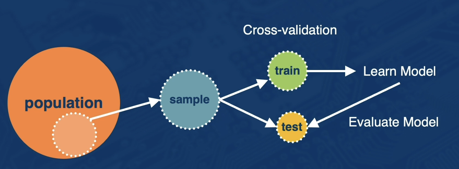
Next, we will walk through each step of the data wrangling process in more detail. So we will first step through what is the population of interest and what sample s are we evaluating and is sample s representative of the population.
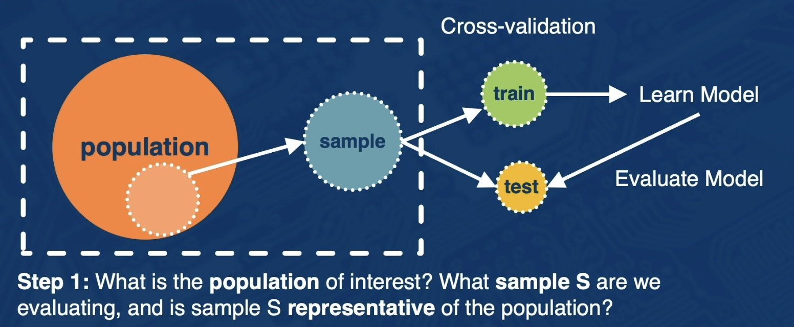
So there are many ways to define target population of interest, here are some examples:
- All Users on Facebook
- All U.S. Users on Facebook
- All U.S users on Facebook that joined in the last month
Next, there are many ways to sample the data and here are just Two sample probability sampling methods
- Simple Random Sampling: every observation from the population has the same chance of being sampled
- Stratified Random Sampling: population is partitioned into groups and then a simple random sampling approach is applied within each group.
Cross Validation and Class imbalanced (optional)
In this portion, we will discuss step 2
- How do we cross validate to evaluate our model? How do we avoid over fitting and data mining?
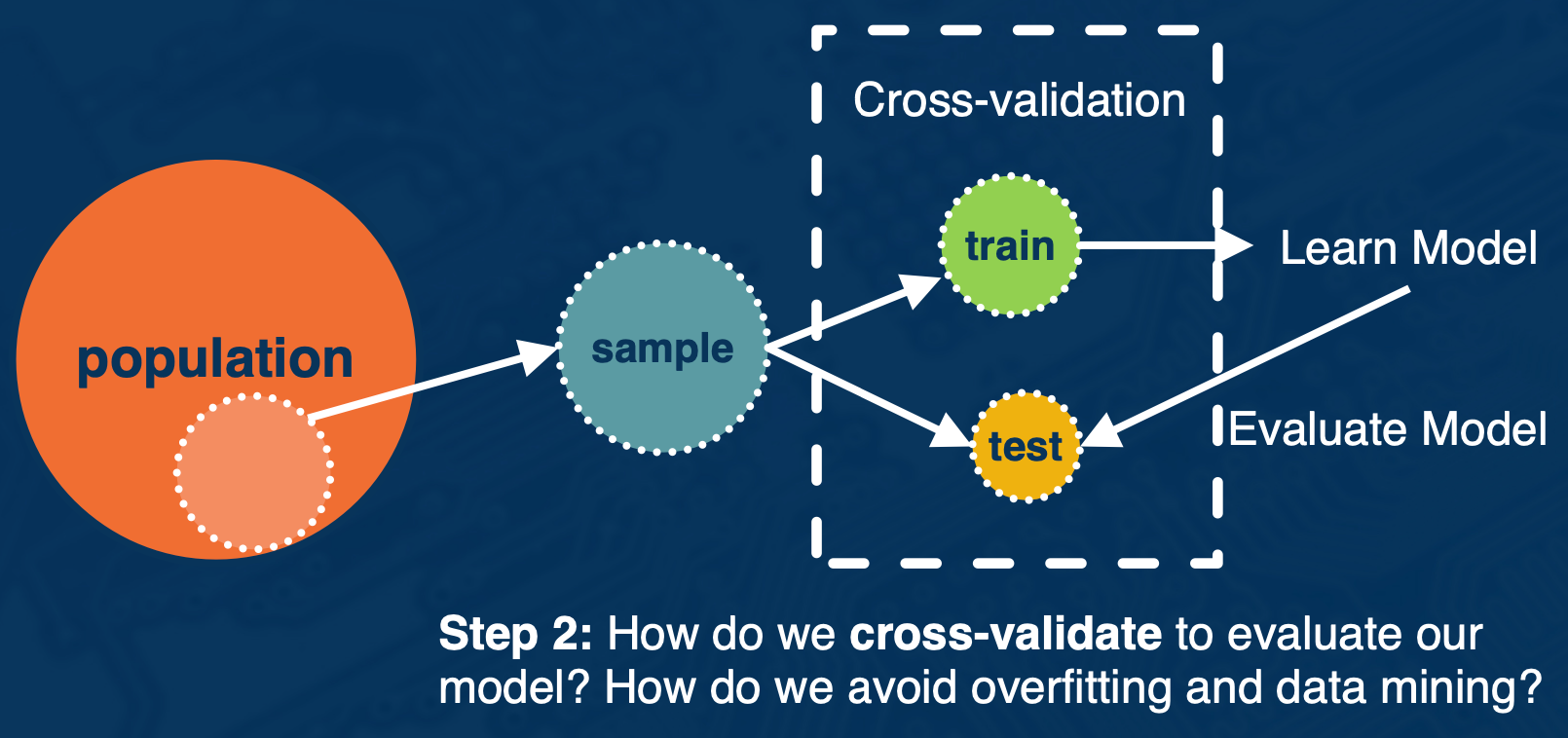
Solution: Use cross-validation.
Best practices
- Random search vs Grid Search for hyper parameters (Bergstra and Bengio)
- Hyperparameter in deep belief networks that random searching can find models at least as good if not better than a grid search in a fraction of the computation time.
- Confirm Hyperparameter range is sufficient (See as an example)
- Temporal (time series) cross-validation considerations
- Future data cannot be used as part of cross validation
- Check for overfitting
Class imbalanced
Class imbalance may occur in binary class prediction settings where one class outnumbers the other class.
Two general ways to address class imbalance in your dataset:
- Sampling base methods
- One popular method is called the synthetic minority over sampling technique or SMOTE.
- Over sampling with replacement the minority class.
- So for each observed minority observation, SMOTE identifies nearest neighbors and feature space will randomly select a subset of these nearest neighbors based on some desired amount of over-sampling. And when we will uniformly sample from the line segment connecting the minority observation and the selected nearest neighbor.
- One popular method is called the synthetic minority over sampling technique or SMOTE.
- Cost sensitive learning methods
Region CNN (R-CNN) and Single Shot Dector (SSD) are models that can localize and classify many objects in an image.They densely sample many boxes of different sizes at different “anchor” locations in the image.

Then for each anchor point, we sample many boxes of different sizes and aspect ratios. These boxes are called proposal boxes. In object detection:
- Goal: Classify a proposal box into foreground or background
- IoU: Intersection over union
- A proposal box is assigned a ground truth label of:
- Foreground, if IoU with ground truth box $> 0.5$
- Background, otherwise.
Cross entropy is a popular loss use for bounding box regression. Easy examples incur a non-negligible loss, which in aggregate mask out the harder, rate examples
\[CE(p,y) \begin{cases} & -log(p), &\text{ if $y=1$} \\ & -log(1-p), &\text{otherwise} \end{cases}\]Focal Loss: down-weights easy examples, to give more attention to difficult examples
\[FL(p_t) = - (1-p_t)^\gamma log(p_t)\]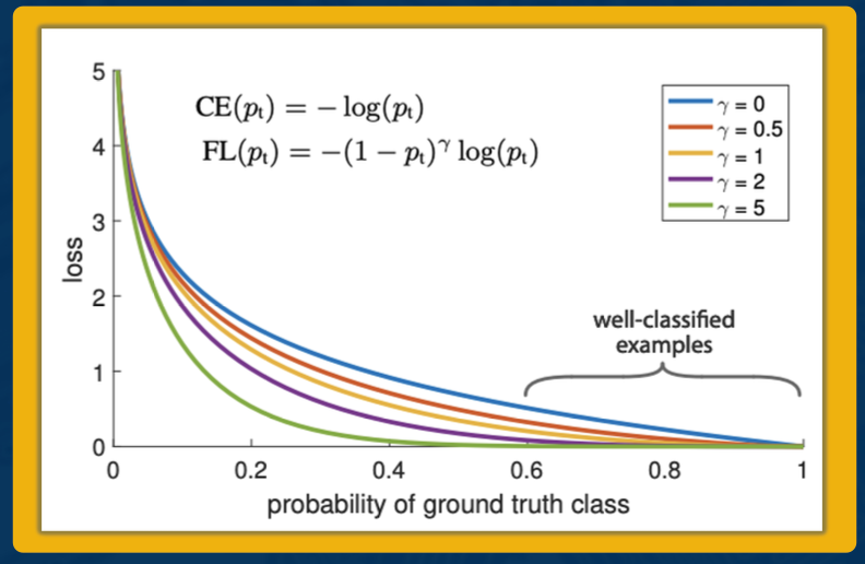
What we mean by easy examples are well classified examples with high probability from the model. The blue line here represents cross entropy, the baseline. You can see, even for higher probability predictions, we still incur a non-zero loss. Compare this to focal loss, where for higher probability predictions, we incur a much smaller loss.
Cross validation done right in class imbalanced settings
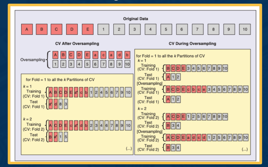
At the top we have our original imbalanced data set. So in red are the minority class, units A through E and in gray, we have our majority class units 1 through 10.
On the left is an illustration of cross-validating after oversampling and this is incorrect. This is because we first over sampled so that we have equal representation of both classes then we cross validate. Lets focus on the k equals 1 split. In both the training and test split, we observe A appearing as indicated by the asterisk. Thats because we oversampled first. So this will lead to an overoptimistic error estimate, since you have data leakage on the same observation appearing on both the train and test split.
Instead the right side illustrates the correct approach to implement cross-validation during oversampling. First the original data is divided into k partitions and only the training split is over sampled. So this is important because it means that no data from the training split will become part of the testing split and we can ensure a fair evaluation.
Prediction and Evaluation (optional)
Model evaluation statistics
- Confusion matrix, metrics
- For regression, you have RMSE etc
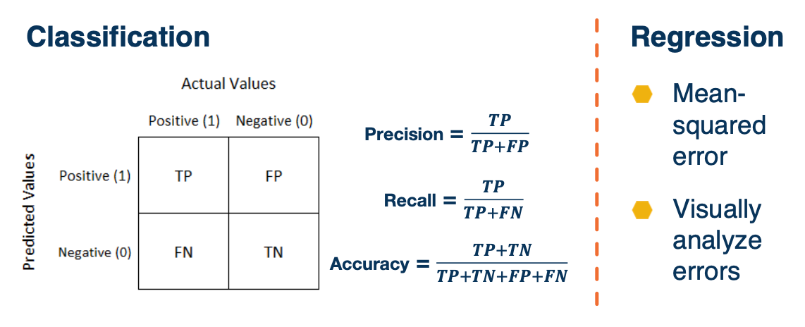
Classification and calibrated Models
For classification models, sometimes it matters not only predicting the class label, but predicting the associated probability. If we care about the classification score that corresponds to a probability score then it can be help to examine calibration plots.
A calibration plot, as shown here, plots on the x-axis the mean predicted value and on the y-axis the fraction of positives. So a perfectly well calibrated plot is shown by the black dotted line where mean predictions are exactly equal to the fraction of positives. A miscalibrated plot is one that deviates from the dotted line. In this plot here we see a logisticregression model as well calibrated, this makes sense since logistic regression is aimed at optimizing the log loss. Meanwhile, we see a support vector classification model is very miscalibrated.
If you find your model is miscalibrated, then there are a variety of options for calibrating such as isotonic regression.
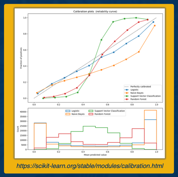
It is important to ask what are we measuring our model performance against?
The importance of baseline - the baseline can be anything:
- Random guessing?
- Current model in production?
- Useful to compare predictive performance with current and proposed model.
summary
- Clearly define your population,
- Understand the representativeness of your sample
- Cross validation can go wrong in many ways; understand the relevant problem and prediction task that will be done in practice
- Know the prediction task of interest (regression vs classification)
- Incorporate model checks and evaluate multiple predictive performance metrics.
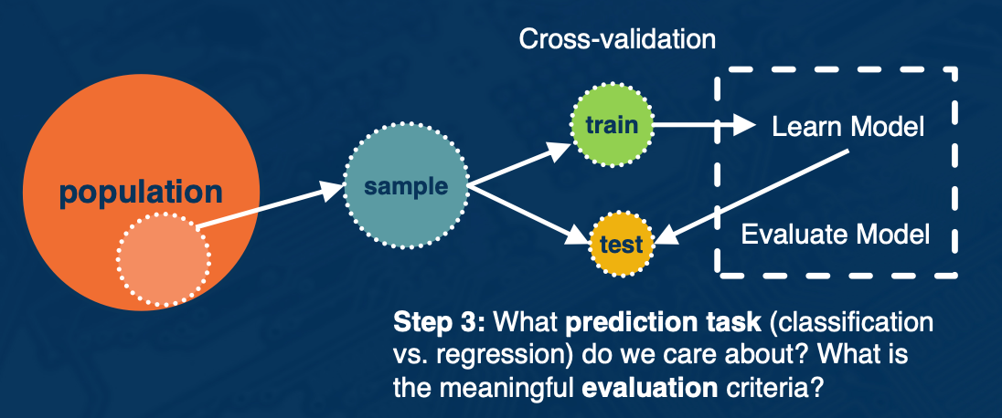
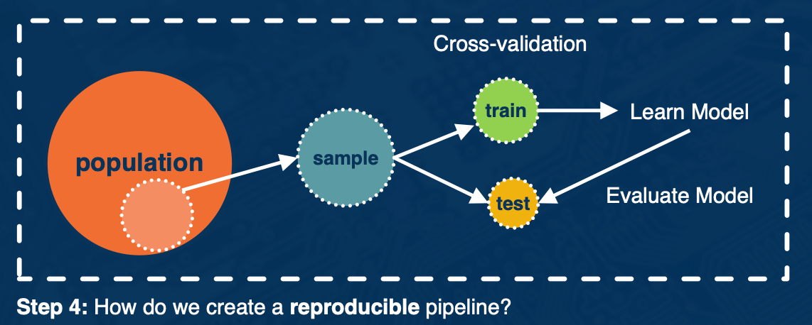
Module 2: Convolutional Neural Networks
Lesson 5: Convolution and Pooling Layers
Readings
Convolution layers
Backpropagation and automatic differentiation, allows us to optimize any function composed of differentiable blocks.
- No need to modify the learning algorithm dependent on what the blocks are
- The complexity of the function is only limited by computation and memory
The connectivity in linear layer doesn’t always make sense. Take images for example, suppose that an image has 1024 by 1024 pixels, when we convert this into a vector, we will roughly have a million parameters. If we put a fully connected layer after it with N nodes, lets say N equals to 1000.
The total parameters is M*N (weights) + N (bias). Hundreds of millions of parameters for just one layer. There are several issues in machine learning with having so many parameters.
- More parameters you have the more data you require
- is this necessary?
Locality of Features
Images features are spatially localized
- Smaller features repeated across the image
- Edges
- Dark pixels vs light pixels tells us whether there are edges in the image. Can repeat this across entire image to extract features.
- Color
- Motifs (corners, etc)
- Small corners, small circular shapes and things like that
- Anything you can detect with a patch of the image and not the entire image itself.
- Edges
- No reason to believe one feature tends to appear in one location vs another (stationary)
- e.g a bird can appear anywhere in the image.
Can use these properties to induce a bias in the design of a neural network to reflect this. By bias, will explore specific connectivity patterns that are more appropriate to images and that will reduce the number of parameters that these layers will have.
Idea 1 - Receptive Fields
Specifically, each node in the neural network only receives input from $\textbf{K_1} \times \textbf{K_2}$ window (image patch).
- Region from which a node receives input from is called its receptive field.
- This node will output the existence of a particular type of feature in that little window for example an edge.
The advantages to this:
- The number of parameters will be reduced to $(K_1 \times K_2 + 1) * N$ where $N$ is the number of output nodes. So we can toggle this by controlling the number of output nodes. This will allow us to have only a certain number of output nodes, each of which only takes input from $K_1$ by $K_2$ image patches.
- Explicitly maintain spatial information.
What about location-specific features?
Idea 2 - Shared weights
Nodes in different locations can share features or weights. Weight sharing means that the specific weights for example, $W_{11}$ for example the left most node is the same for the right most node. The way you can accomplish this is by just having the same variable in the computation graph feed into both of these nodes. So we will have several nodes across the entire output all share weight.
- No reason to think the same feature (e.g edge pattern) can’t appear elsewhere. That edge detection feature will be run across the entire image.
- Using same weights/parameters in computation graph (shared weights)
The advantages:
- Further reduce the number of parameters to $(K_1 \times K_2 +1)$.
- Explicitly maintain spatial information.
Idea 3: Learn many features
We can learn many such features for this one layer. So we may not want to be limited to one type of feature. We can have vertical edges or horizontal edges of lots of things inbetween. At the same time we also want to represent different color features or texture features or corner features or other shapes. And so we will want to have multiple types of features.
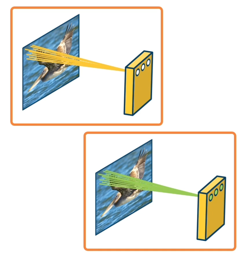
We will have one channel of output, for example on the upper left, that represent locations of features, say edges or a particular edge orientation. This output channel will have nodes with high values in the locations that have such features very strongly. And then on the lower left, we will have another channel of output that represents the location of a different feature.
The weights are not shared across different feature extractors. The weights themselves will represent what type of features we extract from these little windows. But for one particular type of feature on the upper left, all of the nodes are sharing their weights. In other words they are extracting the same type of feature over different locations in the image.
The number of parameters now is $(K_1 \ times K_2 + 1) * M$ where $M$ is the number of features we want to learn.
Convolution
This operation is extremely common in electrical/computer engineering!
In mathematics and, in particular, functional analysis, convolution is a mathematical operation on two functions $f$ and $g$ producing a third function that is typically viewed as a modified version of one of the original functions, giving the area overlap between the two functions as a function of the amount that one of the original functions is translated.
Convolution is similar to cross-correlation.
It has applications that include probability, statistics, computer vision, image and signal processing, electrical engineering, and differential equations.
Notation:
\[F \bigotimes (G \bigotimes I ) = (F \bigotimes G ) \bigotimes I\]1D convolution:
\[y_k = \sum_{n=0}^{N-1} h_n \cdot x_{k_n}\]e.g $y_3 = h_3 \cdot x_0 + h_2 \cdot x_1 + h_1 \cdot x_2 + h_0 \cdot x_3$
2D Convolution:
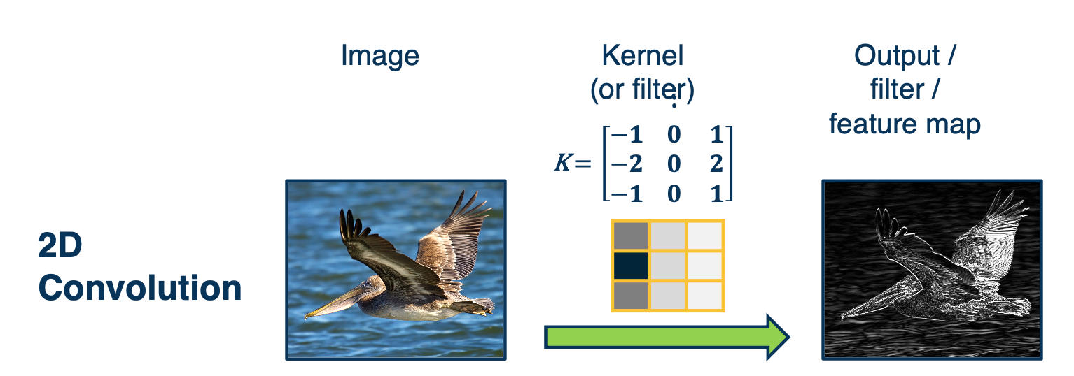
We are mainly interested in 2D convolution.
We will have an image that is fed through what is called a kernel or a filter and get an output or what is called a filter/feature map. In DNN, it is sometimes called an activation map. The output is spatially relevant and maintains spatial information of where the particular kernel or filter is highly expressed in the original image.
Above image is an example to the particular kernel, if we visualize it in grayscale where dark values are very low negative values, and light values are high/positive values. You can see this looks like an edge and this is not a coincidence. This filter will be convolved with image patches, so portions of the image have very dark locations on one side, and very light locations on the other side, this filter will activate very highly. This results in very high values in the corresponding region in the output map.
In Deep learning, we will make this convolution a layer in the neural network.
- Initialize kernel values randomly and optimize them!
- These are our parameters (plus a bias term per filter)
The object is to learn the kernel itself. The output maps after the operation will allow us to classify what is in the image.
Intuitive explanation
What convolution layer is doing is very simple.
We take the kernel and flip/rotate it by 180 degrees. And then take the dot product that kernel with all the different images patches or locations in the image, and add a bias term later.
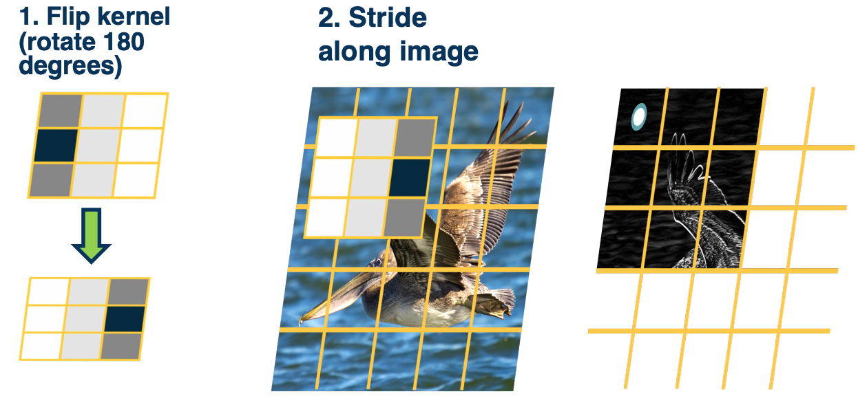
This dot product will result in the value output of the first pixel in the output map, depicted as what that white circle is. Now if you notice if we do it across the entire image, at some point we will run out of room.
Mathematics of Discrete 2D Convolution
Even though the description of what we are doing in the convolution operation is pretty simple, mathematically describing it gets a little hairy. And that is because we need to define coordinate systems for the image and the kernel. And somehow describe mathematically this operation of flipping the kernel as well as striding over the image.
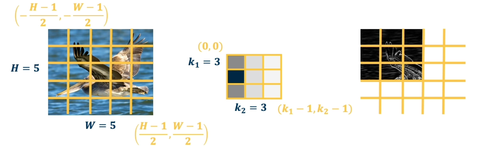
Suppose that we take the image here, simplify it into a 5 by 5 grid, and we will represent a coordinate system where the center pixel is $(0,0)$. And so the upper left is going to be $(-\frac{H-1}{2}, -\frac{W-1}{2})$ and the bottom right is $(\frac{H-1}{2}, \frac{W-1}{2})$.
The kernel coordinate system will be a little different, we will have the upper left defined as $(0,0)$ and the lower right defined as $(k_1-1,k_2-1)$. So lets look at the equation that describes this convolution operation
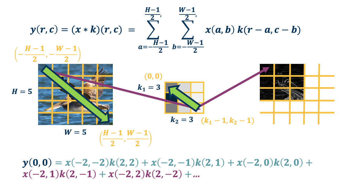
Let’s take the output map $y$, so $y$ represents our output and $(r,c)$ will represent the pixels that are in the output. So $r$ represents the row, and $c$ represents the column, and $(0,0)$ is going to be on the upper left in this case. What we are going to do is $y$ of $(0,0)$ will equal to the summation over the entire image where we dot product or multiply the input pixel the image pixel times the kernel value. But if you look we are summing over the upper left to the lower right all of the pixels in the image, and we are multiplying $x(a,b)$.
So $(a,b)$ is the current pixel in the input image, and multiplying pixel $(a,b)$ in the input image with the kernel value, but the kernel value is not $a,b$ but it is actually $(r-a, c-b)$. This is what is representing mathematically that operation of flipping the kernel.
For example, $y(0,0)$, we iterate over all the pixels in the input image and lets say the upper left which is $x(-2,-2)$. So now $a=-2,b=-2$ And because we are looking at $y(0,0)$ so $(r,c) = (0,0)$. So if you work it out the actual kernel pixel that we are multiplying by is by $r-a$ which is $0-2 = -2$ and the same for the other coordinate. We continue to do this for $x(-2,-1)$ and multiply it by $k(2,-1)$ and so on.
If you notice, at some point you will have negative values for the kernel, and of course you cannot have that since there is no value there. For those cases we just throw those values away.
Convolution and cross correlation
As we have seen:
-
Convolution: Start at the end of the kernel (lower right) and move back towards $(0,0)$
- This is intuitively described as a flipping operation.
-
Cross-correlation: Start in the beginning of the kernel and move forward (Same as for image).
- Very similar to convolution except its applied with the flipped kernel.
An intuitive interpretation of the relationship:
- Take the kernel, and rotate 180 degrees along center (sometimes referred to as “flip”)
- Perform cross-correlation
- Just dot-product filter with image.
Cross-correlation
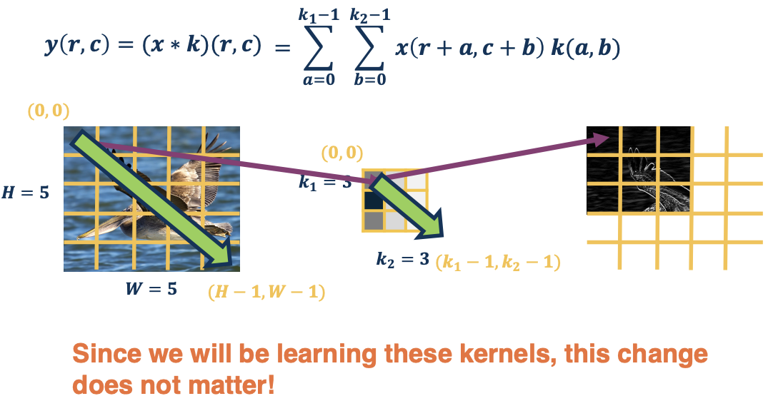
So this is the mathematics of cross-correlation. It is actually a little bit nicer because if you notice rather than having this weird $r-a$, we are now adding things which is a lot more intuitive. And we can have the coordinate systems be the same for both the image and the kernel.
So specifically for the image, we have the coordinate system $(0,0)$ on the upper left, and $(H-1,W-1)$ on the low right and the same thing for the kernel.
One interesting thing is that essentially the pixels is moving in the same direction. That is, the indexing is moving the same direction which makes things a lot more intuitive. This will make backprop equation much simpler.
One interesting thing is that since we are learning these kernels anyway, essentially those kernels are going to be randomly initialized and some learned thing that gradient descent tells us to optimize to. It does not really matter whether you flip the kernel or not. And so, with respect to a learned kernel, there is no real difference between convolution and cross-correlation.
An example:
\[X(0:2, 0:2) = \begin{bmatrix} 200 & 150 & 150 \\ 100 & 50 & 100 \\ 25 & 25 & 10 \end{bmatrix}, K' = \begin{bmatrix} 1 & 0 & -1 \\ 2 & 0 & -2 \\ 1 & 0 & -1 \end{bmatrix}\] \[X(0:2, 0:2) \cdot K' = 65 + \text{bias}\]Why Bother with Convolutions?
Convolutions are just simple linear operations
Why bother with this and not just say it is a linear layer with small receptive field? Why are we bothering with all this mathematical formulation of what a convolution is, as well as describing the relationship between the convolution and cross-correlation?
- There is a duality between convolution and cross-correlation during backpropagation
- It turns out that when you do the forward pass as a cross-correlation, which is actually how we will implement it, because that is the easy thing to implement, and it is also easy to vectorize. It turns out when we compute the gradients which we will go through, it actually will be a convolution
- If you forward pass a convolution, the backwards pass will be a cross-correlation. So it is good to know the relationship just because of that.
- Convolutions have various mathematical properties that people care about
- For example we can take the kernels that are learned when we do cross-correlation, and we can then flip them and describe them as a convolution and maybe do some analysis.
- This is historically how it was inspired.
Input and Output Sizes
A convolution layer as we described is taking a kernel of a particular size and striding it over the image and doing a dot product across all the locations to produce a spatially organized output map.
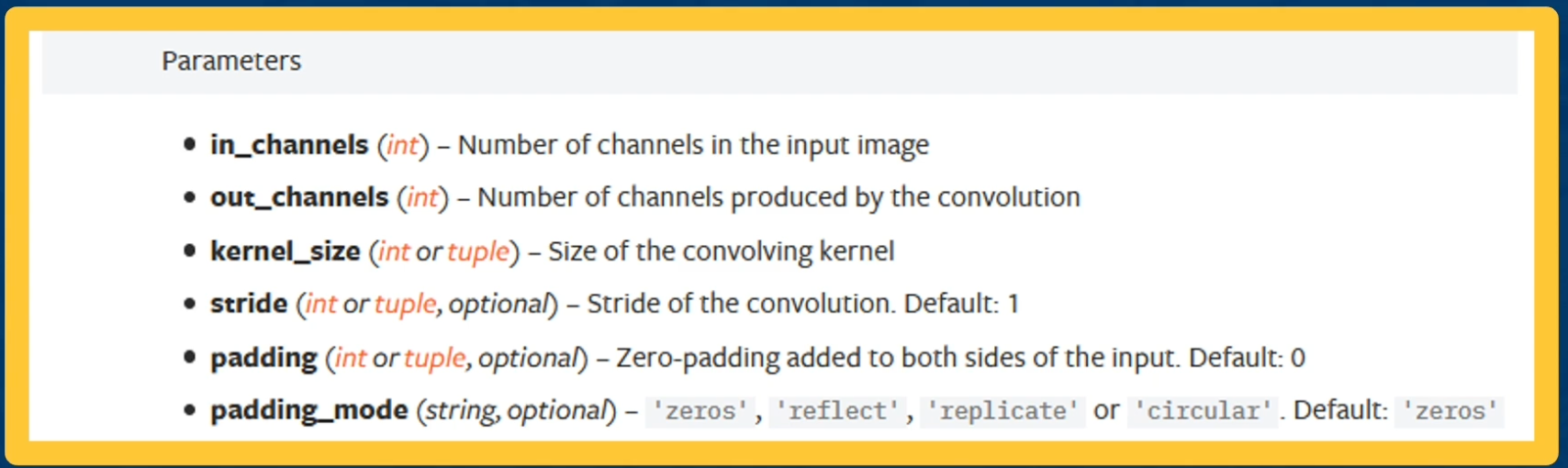 https://pytorch.org/docs/stable/generated/torch.nn.Conv2d.html
Now there are several design decisions or hyper parameters that exists for these layers.
- Input Channels - For example in an image, we can have three channels - the RGB
- Output channels - how many kernels we use.
- Kernel size - we can have 3 by 3 as shown or any size you want. They do not have to be square either
- Stride - We also have the stride that is we will move the kernel along the image, not one pixel at a time but a few pixels at a time.
- Padding - can pad the image or surround by zeros in order to change the output size.
Valid Convolution
The output size of a vanilla convolution operation is just the dimension of the image minus the dimension of the kernel plus one $(H-k_1+1) \times (W - k_2 + 1)$
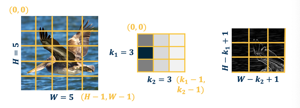
So in the above example, we will have a three by three output map. To repeat, the reason it is smaller is because if we move that kernel over more than three times, for example the fourth time, the kernel goes off the image.
So a valid convolution is only when the kernel is fully on the image.
Adding Padding
We can also pad the images to make the output the same size. In some cases, we want to have one input size and then have the same output size. What we can do is just surround the image with zeros but there are also other things that we can do, for example we can mirror the image.
For example the pixels at the border will be reflective of the pixels in the actual image across the border.
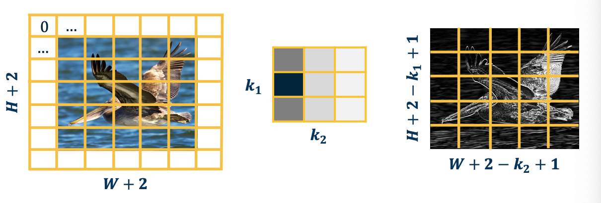
Note that padding often refers to adding one dimension, so $P=1$ or padding size of one here is shown but actually you are adding two to the height because you are going to add a padding to the bottom as well as the top
Stride
We can also move the filter along in larger step sizes than just one (stride).
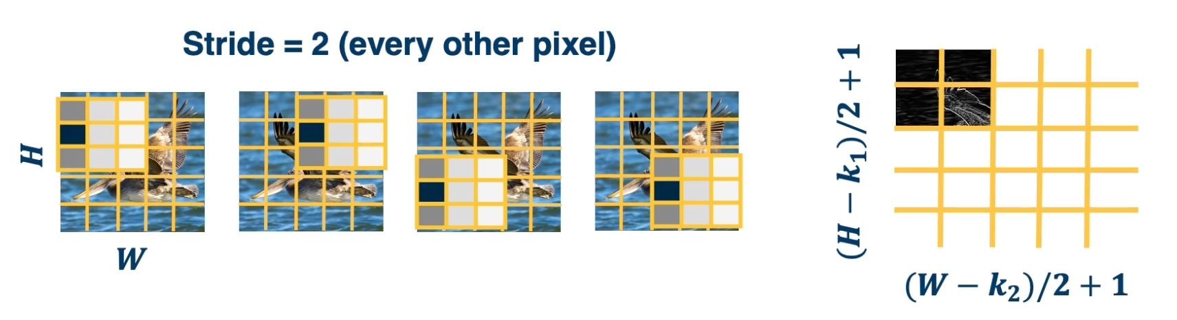
- This can potentially result in loss of information.
- Can be used for dimensionality reduction (not recommended)
Note that some combinations are not going to be valid and cna result in skip pixels at the edge. For example a stride of 3 for 5x5 input with a 3 by 3 kernel.
Multi Channel inputs
We talked about one channel inputs, such as greyscale images, but in reality they have three channels (red green blue). So we will have a tensor of size height by width by three. So in that case, how do we design the kernel for the convolution operation?
It turns out we can just have a three channel kernel, i.e the depth of the kernel extended to be equal to the depth of the input.
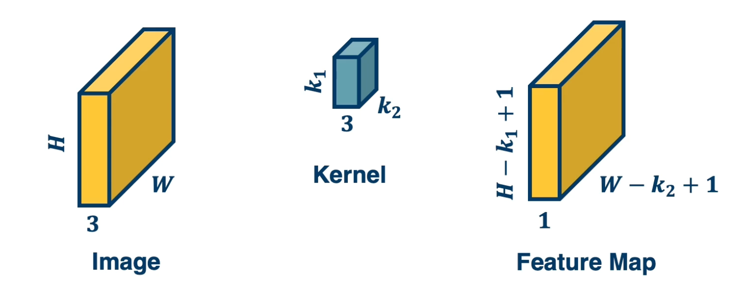
We actually do the same dot product operation, except rather than do it with three by three values, instead do it with three by three by three values.
The following image depicts how we can do this:
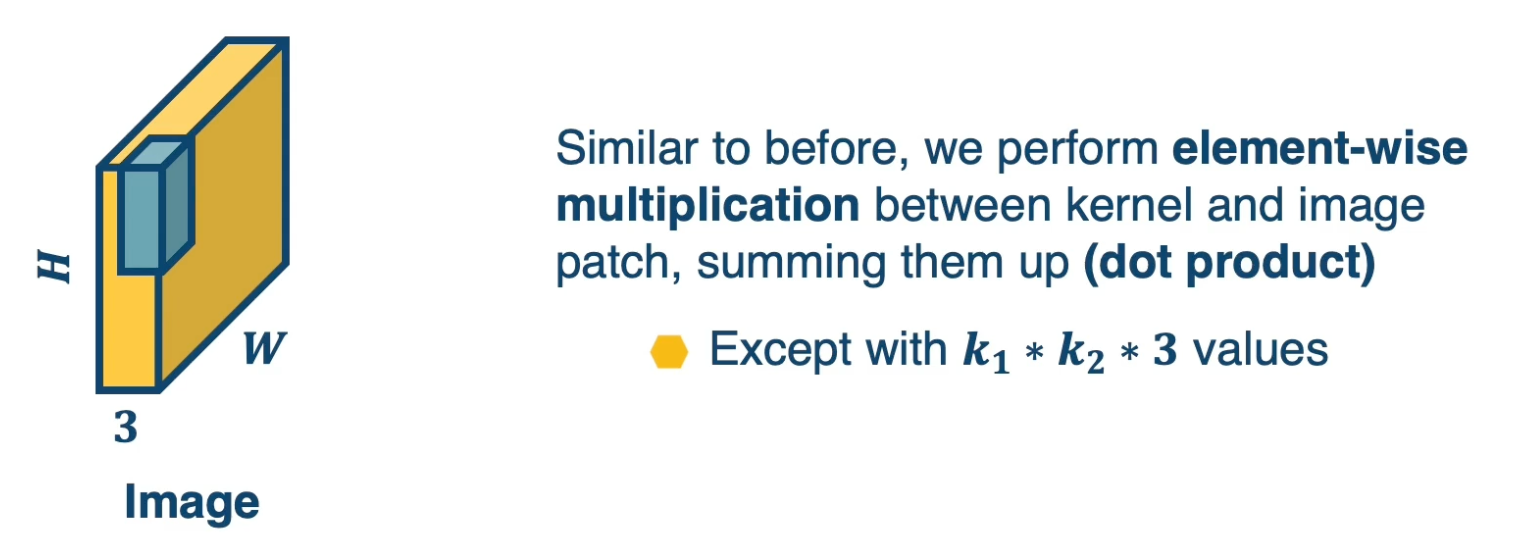
We can also have multiple kernels per layer. This is because we want multiple feature extractors for each image. These kernels could represent things like edges of a particular orientation so it is good to have many of them. We will also want kernels that represent extraction of color features or texture features and so on. Remember, it is gradient descent that will learn these kernels.
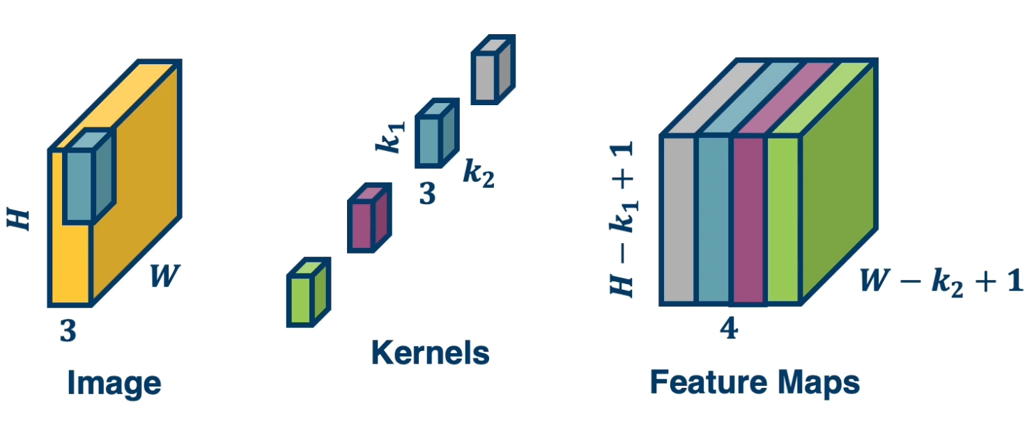 stack the feature maps together at the output, remember the number of channels in output is equal to the number of kernels
Then there is a question of why you will not learn the same exact type of features? It turns out the reason is we initialize them to different values so all of these kernels will initialize the different values and their local minima in their local weight space will be different and so they will end up learning different features.
The gradient for each kernel will be different because we initialize them differently and they will move in different directions. You might have redundancy in this case and we will see this when we visualize what this network will learn.
Now let’s take a look at the number of parameters (recall that the idea of using convolution is to reduce the number of parameters.). In the above image, assume that each filter is $k_1 \times k_2 \times 3$, that is how many parameters we will have because each of those values in the kernel is the parameter that we are learning and initialize randomly. We will have a plus 1 here again for the bias. So if we have $n$ kernels, then the total parameters is $N * (k_1 * k_2 * 3 + 1)$
Vectorization of Convolution
Just as before, in practice we can vectorize this operation.
- Step1: Lay out images patches in vector form.
- Step 2: Multiply patches by kernels
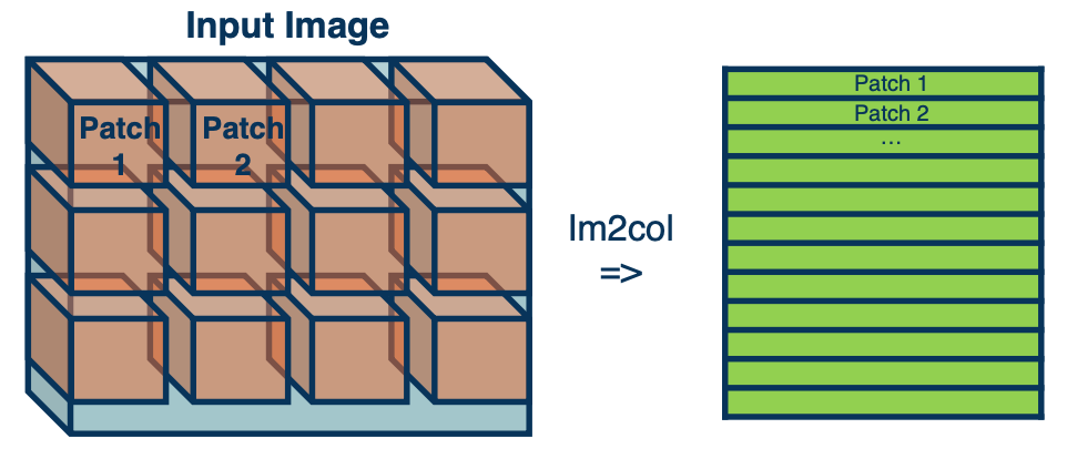
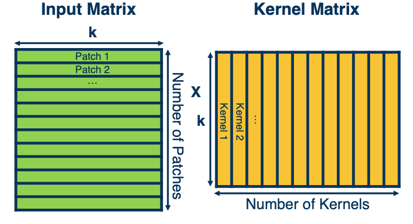
Pooling layers
In this lesson we will introduce a new layer called the pooling layer that can perform dimensionality reduction. That is down sampling things like images.
-
Dimensionality reduction is an important aspect of machine learning.
- As we know, we often have very high dimensional input and we do not actually need to characterize those high dimensional inputs in as much information.
- That is we can compactly represent the important information, for example, for the task of classifying within the image.
- Can we make a layer to explicitly down-sample image or feature maps?
- Yes! We call one class of these operations pooling operations
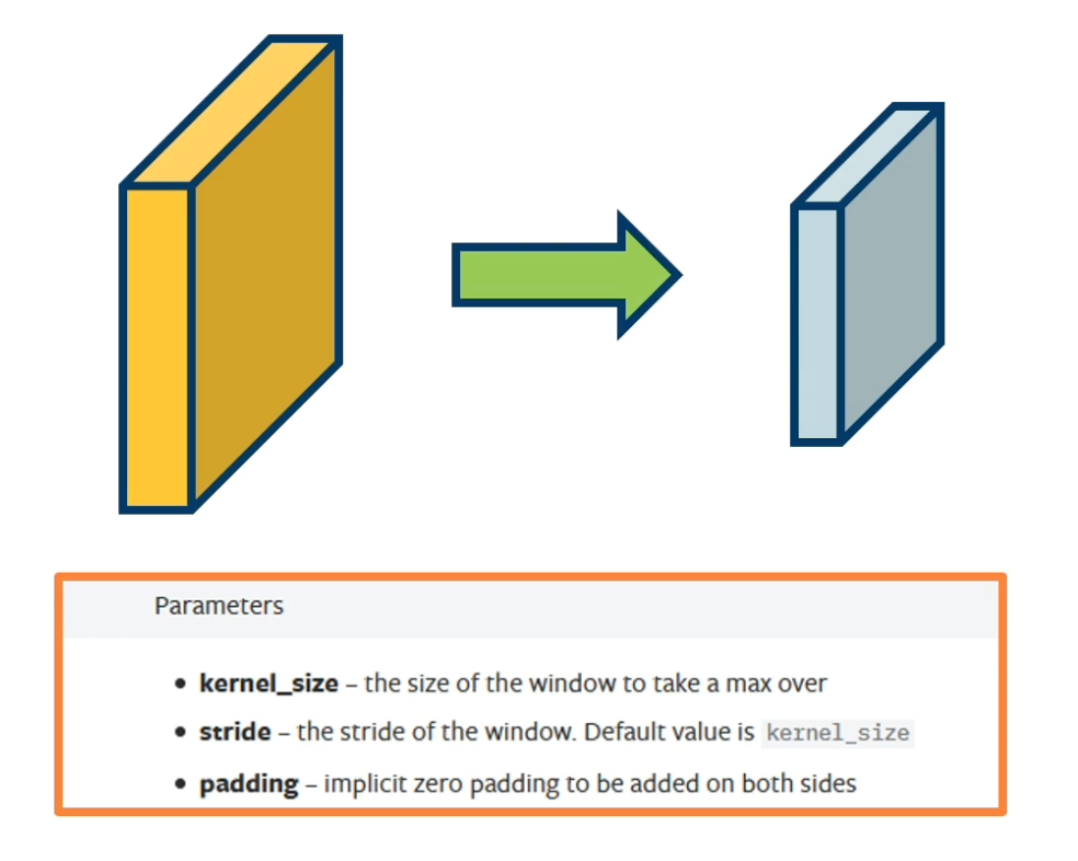 https://pytorch.org/docs/stable/generated/torch.nn.MaxPool2d.html
Max pool layer
Example: Max pooling
- Stride window across image but perform per-patch max operation
How many learned parameters does this layer have? None!
Not restricted to max: can use any differentiable function, such as average (Not very common in practice), typically we use max operation. You will see in much later neural network architectures we might get rid of the pooling layer all together and perform dimensionality reduction using convolutions themselves.
\[X(0:2, 0:2) = \begin{bmatrix} 200 & 150 & 150 \\ 100 & 50 & 100 \\ 25 & 25 & 10 \end{bmatrix}\] \[avg(X(0:2,0:2)) = \frac{1}{N}\sum_i \sum_j x(i,j) = 90\]Combining convolution and pooling layers
Since the output of convolution and pooling layers are (multi channel) images (i.e a tensor), we can sequence them just as any layer. For example, we can take an image, perform a convolution to get an output channel or image and then apply pooling to that same output. We can continue to sequence these layers over and over again.
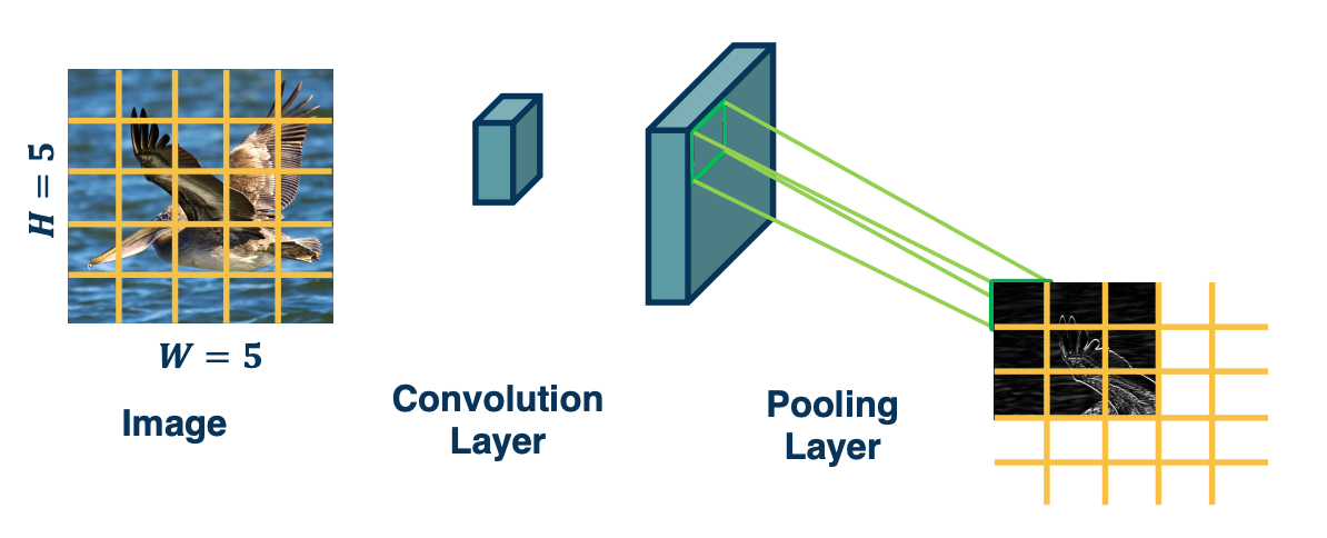
Invariance
This combination where we perform a convolution and then a pooling actually has a powerful feature. Specifically it results in what is called invariance
- if the feature (for example a beak) translated a little bit, output values may still remain the same
- This is because the kernel - the feature that picks out beak will have a high value that moves a little bit in the output map.
- But if we move within the pooling window, that is as long as the movement is not much larger than the size of the pooling window, then the max across that window will still be the same. And so if there is a high value there because there was a beak there, then we will still have a high value after pooling.
- So movements, at least slight movements of the features themselves in the input image will result in the same exact value in the output map.
- This is what is called invariant
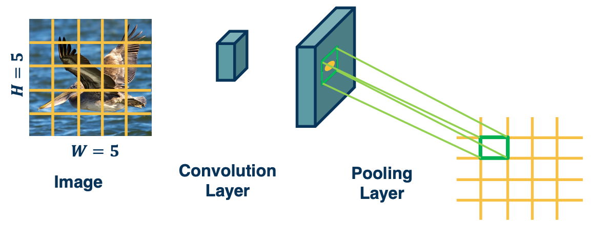
Invariance vs Equivariance
Convolution by itself has the property of equivariance. This is something that convolution operations naturally have even without pooling.
- If feature (such as beak) translated a little bit, output values move by the same translation
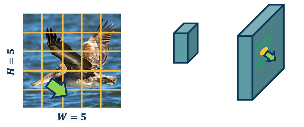
For example if the beak feature or pixels move a little bit, then the kernel will st ill stride across the entire image and pick it up in that new location. So it will have high output value in that new location. This means that in the output map, the high value moves in the same direction as the actual feature in the image.
Both of these types of features are actually quite important, for example in terms of invariants, we want various transformations or things like translation or rotation to not affect the output very much. Eventually at least deep in the network when we start to do classification we do not want the classification outputs to change very much. We still want this bird to be classified as a bird even though the beak feature moved. So, having these equivariance and invariance properties are actually very important.
Lesson 6: Convolutional Neural Network Architectures
Readings
None!
Backwards Pass for Convolution Layer
It is instructive to calculate the backwards pass of a convolution layer even though in practice, automatic differentiation will do it for us.
- Similar to fully connected layer, will be a simple vectorized linear algebra operation!
- We will see a duality between cross-correlation and convolution
As a reminder: here is the cross correlation operation:
\[y(r,c) = (x*k)(r,c) = \sum_{a=0}^{k_1-1} \sum_{b=0}^{k_2-1} x(r+a,c+b)k(a,b)\]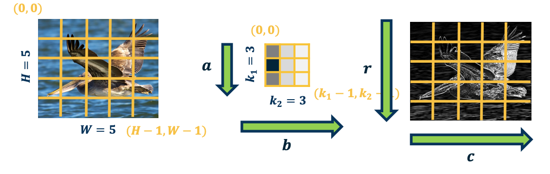
Some simplifications: 1 channel inp ut, 1 kernel (channel output), padding (here 2 pixels on right/bottom) to make output the same size.
The output map $\lvert y \lvert = \textbf{H} \times \textbf{W}$ is going to be height by width, this is the same size as the input. So the upstream gradient, the partial derivative of the loss with respect to our output for this convolution layer is given by whatever layer is after this one and we are going to assume some things about it.
- $\frac{\partial L}{\partial y}$ - Assume size $H \times W$ (add padding, change convention abit for convenience)
- $\frac{\partial L}{\partial y(r,c)}$ - to access element of a particular pixel of the jacobian.
Just like any other layer, we will define the convolution layer as some black box that has an input, output nad a set of parameters.
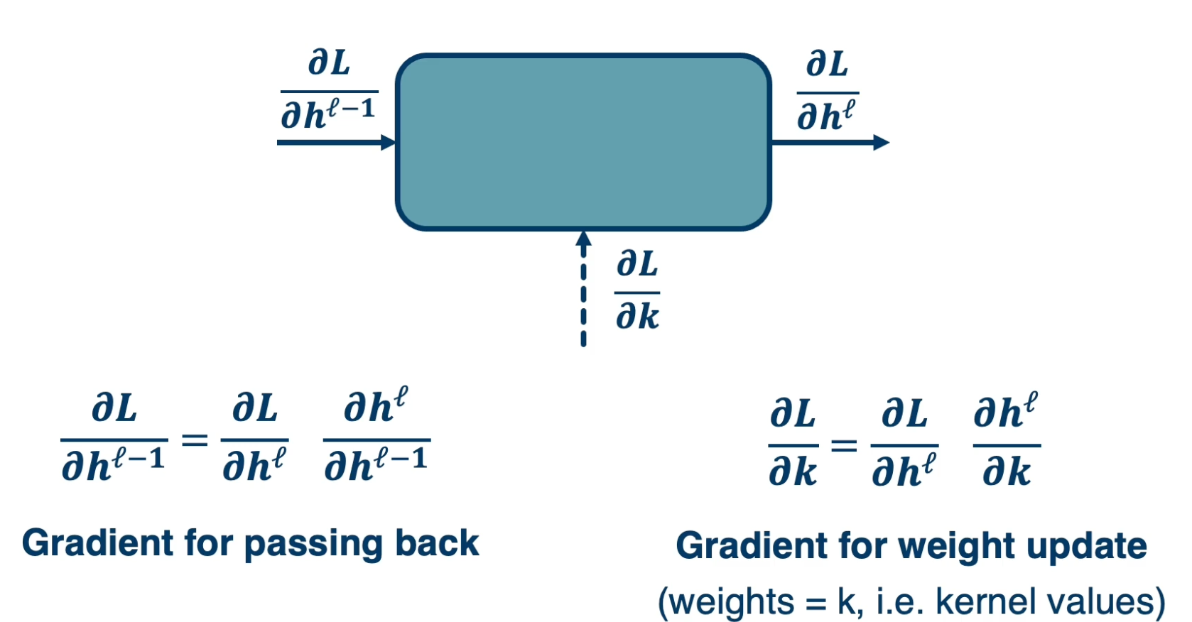
Specifically it has an input $h^{l-1}$, typically some tensor, an output $h^l$ where the depth is equal to the number of kernels in the layer, and $w$, the learnable parameters. In this case, the parameters are the kernel values themselves.
We want to compute the partial derivative of the loss, with respect to our input, $h^{l-1}$ as well as with respect to our weights (kernel values) in order to update them. While we want to do this based on the upstream gradient that were given from whatever module exists after this one. That is the partial derivative of the loss, with respect to our output and is something we are given.
If you remember, we will use the chain rule to compute this, the partial derivative of the loss with respect to our input will just be equal to the partial derivative of the loss with respect to our output times the partial derivative of the output with respect to our input. This is saying that if we know how the loss changes as our output changes in small ways and we know how our output changes if our input changes in small ways, then we can multiply those contributions and get the ultimate change of the loss with respect to our inputs. Similarly, the partial derivative of the loss with respect to our weights, again uses this chain.
Gradient for Convolution Layer
In this lesson, we will derive the gradients for the convolution layer and show interesting characteristics derived from it, and how it can be implemented efficiently just like any other layer using linear algebra operation.
What a Kernel Pixel Affects at Output
Let’s start with the gradients for the weight update. Specifically we can do this one pixel at a time. That is, the partial derivative of the loss with respect to $W(a,b)$ or $\frac{\partial L}{\partial k(a,b)}$
![]()
So what does this weight affect at the output? Because if you remember, the forward paths induces a computation graph where this particular pixel $W(0,0)$ performs some effect on the output. This can be multiple outputs, you can see it as multiple edges coming from this pixel in the kernel to the output map. And so for each edge that is outgoing from this pixel, we want to have a corresponding backwards edge through which gradients flow.
So, what do you think this weight affects at the output? Which of the pixels in the output does it affect? The answer is Everything!!. This is because we are striding the kernel across the input image. So in the first location, the first pixel in the input $x(0,0)$ is multiplied by $W(0,0)$. And that gets summed with the other contributions to result in that output map $y(0,0)$. But then we move the kernel over one spot and again it is weight shared, so there is another out going edge where we are now multiplying $W(0,0)$ with $x(0,1)$ and that gets contributed to the output of $y(0,1)$ and so on. As we continue to do this, if you think about it, that one kernel pixel is affecting the entire output. IF we change that one kernel pixel, it will actually change the entire output map, at least by a little bit.
Chain Rule over all Output pixels
Because this one kernel value affects all of the pixels on the output, we actually need to incorporate all of the upstream gradients. That is, partial derivative of loss with respect to $y(0,0), (0,1)$ and so on all the way to the end:
\[\bigg\{ \frac{\partial L}{\partial y(0,0)}, \frac{\partial L}{\partial y(0,1)}, ..., \frac{\partial L}{\partial y(H,W)}\bigg\}\]The way we can do this is through the chain rule. Again, if you have an outgoing arrow in the computation graph from a particular variable, and that variable affects multiple things at the output, then we will just sum the gradients where we perform the backwards pass. That is, you will have a corresponding backwards edge back to the same variable and you will add all the gradients across all the edges. And so this is what it looks like:
\[\frac{\partial L}{\partial k(a',b')} = \sum_{r=0}^{H-1} \sum_{c=0}^{W-1} \frac{\partial L}{\partial y(r,c)} \frac{\partial y(r,c)}{\partial k(a',b')}\]We will have the partial derivative of the loss with respect to $W(a’,b’)$ is equal to the summation across the entire output map. And for each pixel, we will use the chain rule locally. We will do the partial derivative of the loss with respect to that pixel (this is given to us via upstream gradient) times the partial derivative of the output pixel with respect to particular kernel.
\[\frac{\partial L}{\partial k(a',b')} = \underbrace{\sum_{r=0}^{H-1} \sum_{c=0}^{W-1}}_{\text{sum over pixels}} \underbrace{\frac{\partial L}{\partial y(r,c)}}_{\text{known}} \underbrace{\frac{\partial y(r,c)}{\partial k(a',b')}}_{\text{compute}}\]So, how do we calculate this term? You can do this analytically or visually. In this case, let’s do it visually. On the bottom, you can actually see that when we have a pixel $(r,c)$ at the output and we are applying a particular kernel pixel, $(a’,b’)$, and actually there is a question of what is the input pixel that is multiplied by it?
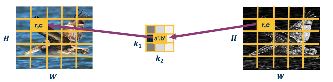
When we actually have the kernel pixel, $(a’,b’)$, which input pixel is multiplied by it? The reason we want to know is we are trying to take the derivative.
Gradients and Cross-Correlation
\[\frac{\partial y(r,c)}{\partial k(a',b')} = x(r+a', c+b')\]We are looking at the output pixel $(r,c)$ and a particular arbitrary kernel $(a’,b’)$, the actual input pixel which gets multiplied by and hence is the derivative is $x(r+a’, c+b’)$. One way to easily do this is just think of the extremes, when $a’,b’$ are both 0, then we just get $x(r,c)$ which is visually what is depicted here. If we move it one to the right and one down, then we get $r+1, c+1$ and so on.
\[\therefore \frac{\partial L}{\partial k(a',b')} = \sum_{r=0}^{H-1} \sum_{c=0}^{W-1} \frac{\partial L}{\partial y(r,c)} x(r+a', c+b')\]This equation is actually a cross-correlation between upstream gradient and input until $k_1 \times k_2$ output.
Forward and Backward Duality
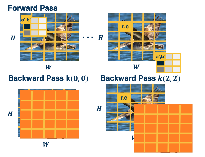 Orange picture is $\frac{\partial L}{\partial y}$
In the forward path, we are striding this kernel across the image and we have some particular kernel value that we care about $(a’,b’)$ and we want to compute the backward pass for that. When $(a’,b’)$ is $(0,0)$, this is showing the cross-correlation that we will be doing. We are actually just cross-correlating literally the input and the upstream gradient, partial derivative of the loss with respect to our output (which is a matrix of size H by W). For the backward pass of $k(2,2)$, this is showing what we are cross-correlating.
What an Input Pixel Affects at Output
Now that we have the gradients with respect to our weights, let’s calculate the gradients with respect to our input. The reason we need this is not to update the weights for this layer, but to pass back to whatever previous layer occurred before this one.
\[\frac{\partial L}{\partial x } = \frac{\partial L}{\partial y } \frac{\partial y}{\partial x }\]What we want to do is let’s calculate this pixel one at a time, $\frac{\partial L}{\partial x(r’,c’) }$. We can try to think what does this input pixel affect at the output? If you think about it and visualize striding the kernel around the input image producing the output, what you will notice is that there is several positions where the particular kernel touches this pxiel. And whenever the kernel touches the pixel that means that the pixel gets incorporated into the output through the summation. That means if I change this particular input pixel then the output pixel will change. Which means that there should be a gradient. So, I can try to reason, about what the neighborhood is affected at the output. This is because I need to chain rule it with the partial derivative of the loss with respect to the particular pixel.
Extents at the Output
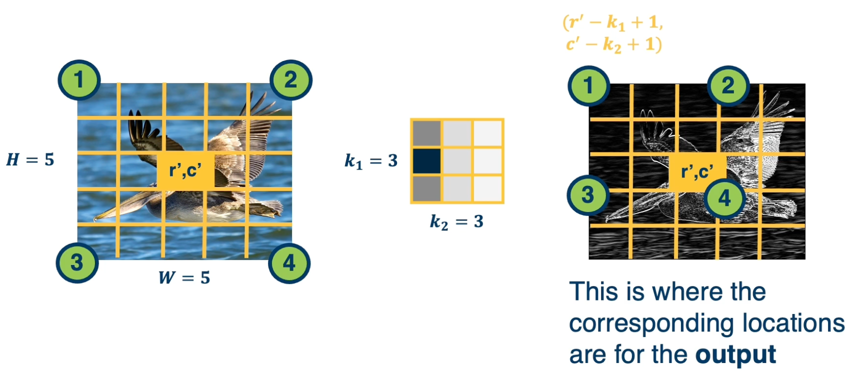
We can try to reason at these four extremes and the input side which parts of the output does it touch. The reason we care about this is we are applying the chain rule and we need to know which elements of the upstream gradient that we get. Should we actually use it in the chain rule?
The four extreme points on the input correspond to these four extreme points on the output. That is point four, which is where the kernel position $(0,0)$ touches $r’,c’$. It actually corresponds to $r’,c’$ on the outputs. And so again, these are the four points on the output where the corresponding locations are for these particular pixel.
Summing Gradient Contributions
Now that we know all the positions on the output map that are affected, we can compute the chain. That is we can compute the partial derivative of the loss with respect to this particular input pixel $r’,c’$ as the summation of all the affected pixels on the output and sum all the chain rules. That is, partial derivative of the loss with respect to y of the affected pixel times the partial derivative of the affected pixel at the output with respect to this particular input pixel $r’,c’$. Again, the reason we are summing up all the gradients us because you can see this as a computation graph where this particular pixel in the input $(r’, c’)$ has an outing edge to multiple output pixels. And so for each of those output pixels, we want to calculate it’s effect and calculate the backwards gradient going through that edge. And so we can try to figure out what should these actual pixels be?
\[\begin{aligned} \frac{\partial L}{\partial x(r',c')} &= \sum_{\text{pixels p}} \frac{\partial L}{\partial y(p)} \frac{\partial y(p)}{\partial x(r',c')} \\ &= \sum_{a=0}^{k_1-1}\sum_{b=0}^{k_2-1} \frac{\partial L}{\partial y(r'-a, c'-b)} \frac{\partial y(r'-a, c'-b)}{\partial x(r',c')} \end{aligned}\]This shows the particular pixels that are affected on the output. Specifically, if you think about it, when you have kernel pixel $(a,b)$ equal to $(0,0)$, then you have the output pixel $y(r’,c’)$ . That is, when the input pixel $r’,c’$ touches the kernel pixel $(0,0)$, that kernel is all the way to the right and all the way to the bottom. Similarly, when the kernel is all the way to the upper left, that means you are multiplying the input pixel $r’,c’$ times the lower right of the kernel. So that is why you subtract $(r’-a, c’-b)$. And so this is the final chain rule or set of chain rules that we are going to sum in order to compute the gradient with respect to this particular input pixel. Again, the partial derivative of $\frac{\partial L}{\partial y(r’-a, c’-b)}$ is given to us, we are given the entire matrix or jacobian. And so all we need to compute is the right side, partial derivative $\frac{\partial y(r’-a, c’-b)}{\partial x(r’,c’)}$…
Lets drive it analytically this time ( as opposed to visually)
Calculating the Gradient
Definition of cross-correlation (use $a’,b’$) to distinguish from prior variables. The reason is that we already define $a$ and $b$ as iterators over the kernel in the previous section.
\[\begin{aligned} y(r',c') &= (x*k)(r',c') \\ &= \sum_{a=0}^{k_1-1}\sum_{b=0}^{k_2-1} x(r'+a',c'+b')k(a',b') \end{aligned}\]Plugin what we actually wanted:
\[\begin{aligned} y(r'-a,c'-b) &= (x*k)(r',c') \\ &= \sum_{a=0}^{k_1-1}\sum_{b=0}^{k_2-1} x(r'-a +a',c'-b+b')k(a',b') \end{aligned}\]Then,
\[\frac{\partial y(r'-a,c'-b)}{ \partial x(r',c')} = k(a,b)\]The reason is that we want the term with with $x(r’,c’)$ in it and this happens when $a = a’, b=b’$.
Backwards is Convolution
Plugging in to earlier equation:
\[\begin{aligned} \frac{\partial L}{\partial x(r',c')} &= \sum_{a=0}^{k_1-1}\sum_{b=0}^{k_2-1} \frac{\partial L}{\partial y(r'-a, c'-b)} \frac{\partial y(r'-a, c'-b)}{\partial x(r',c')} \\ &= \sum_{a=0}^{k_1-1}\sum_{b=0}^{k_2-1} \frac{\partial L}{\partial y(r'-a, c'-b)} k(a,b) \end{aligned}\]This is actually just a convolution between the upstream gradient and the kernel. This can be implemented efficiently rather than performing the convolution we can actually just perform the cross-correlation, but we need to flip the kernel here. And so we can just implement the kernel flipping and cross correlation and all of these operations can be implemented via matrix multiplication.
If we perform a cross-correlation in the forward path, then the particular gradient with respect to the input is actually a convolution which is pretty interesting.
Simple Convolutional Neural Networks
Since the output of convolution and pooling layers are (multi-channel) images, we cna sequence them just as any other layer.
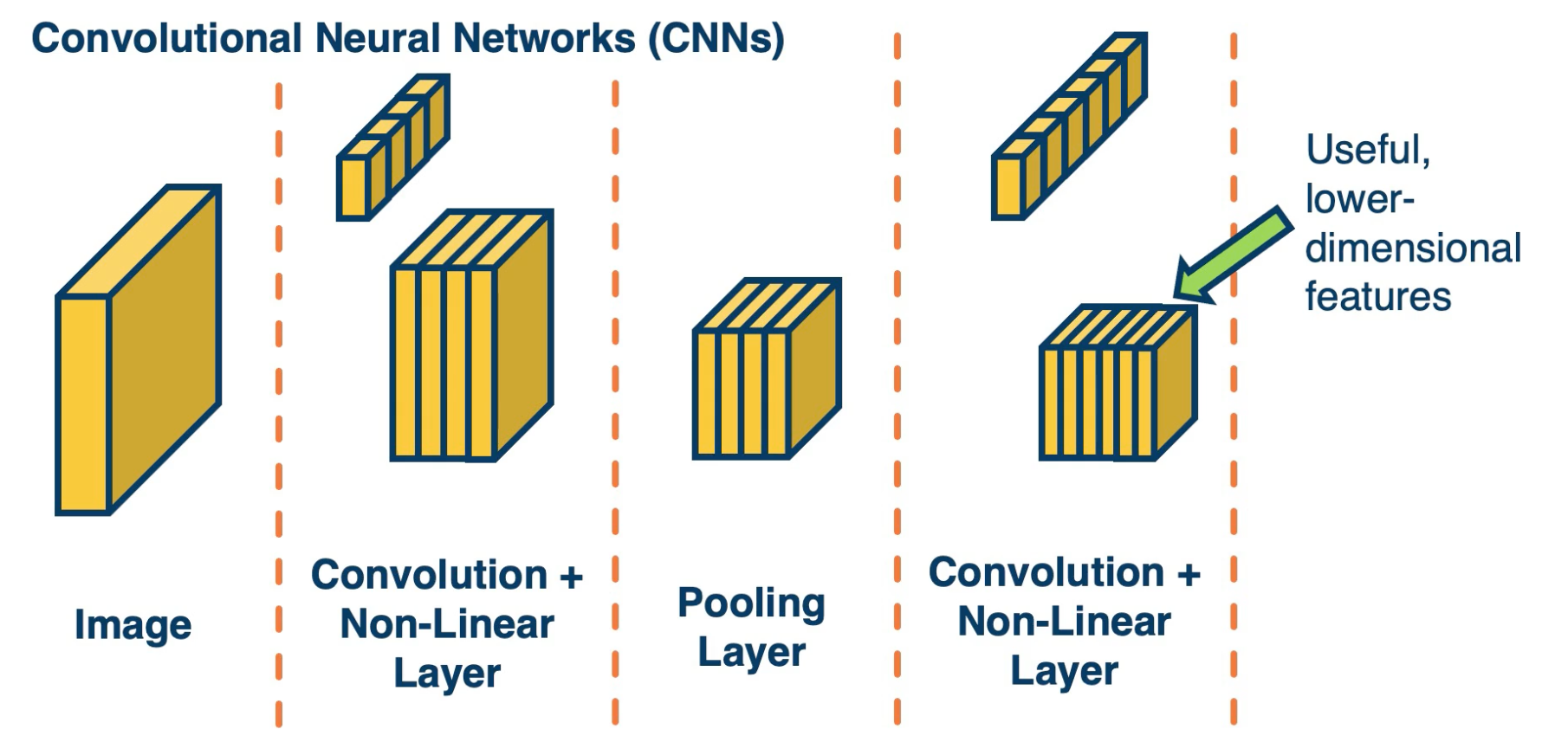
Take the last few layers, and if we optimize to reduce some loss, will hopefully represent more abstract features the deeper we go in this neural network.
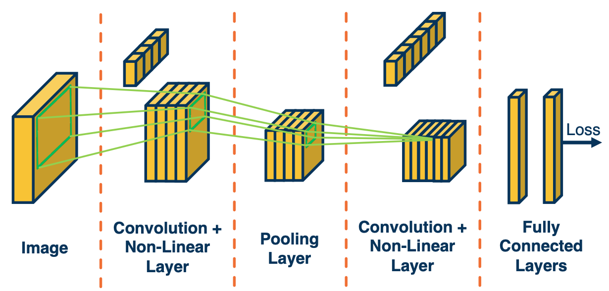
Typically, we will take these last feature maps and feed them through fully connected layer and eventually feed it to a loss function (such as cross entropy).
One interesting aspects of alternating these types of layers is that you will have an increasing receptive field for a particular pixel deep inside the network. Again the receptive field defines what set of input pixels in the original image affect the value of this node or activation deep inside the network. If you see the depiction here, a particular pixel in the output map, in the last convolution layer here is affected by a small window around it in the previous layer. But each of those pixels in this small window are affected by some window around it in the previous layer before that, and you can keep going back over and over.
This will be important later when we start designing interesting convolution neural network architecture.
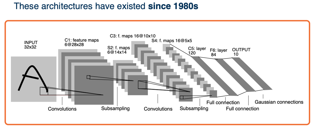 (Gaussian connections just corresponds to a mean squared error loss function - this was back then when we did not use cross entropy)
CNN that existed since 1980 and these have been processing bank checks to perform optical character recognition for quite a while now.
We will now look at other more advance architectures.
Advanced Convolutional Networks
As data availability increases, so does complexity increases and hence more complicated neural networks. An example was the ImageNet competition where neural network blew the competition away.
AlexNet
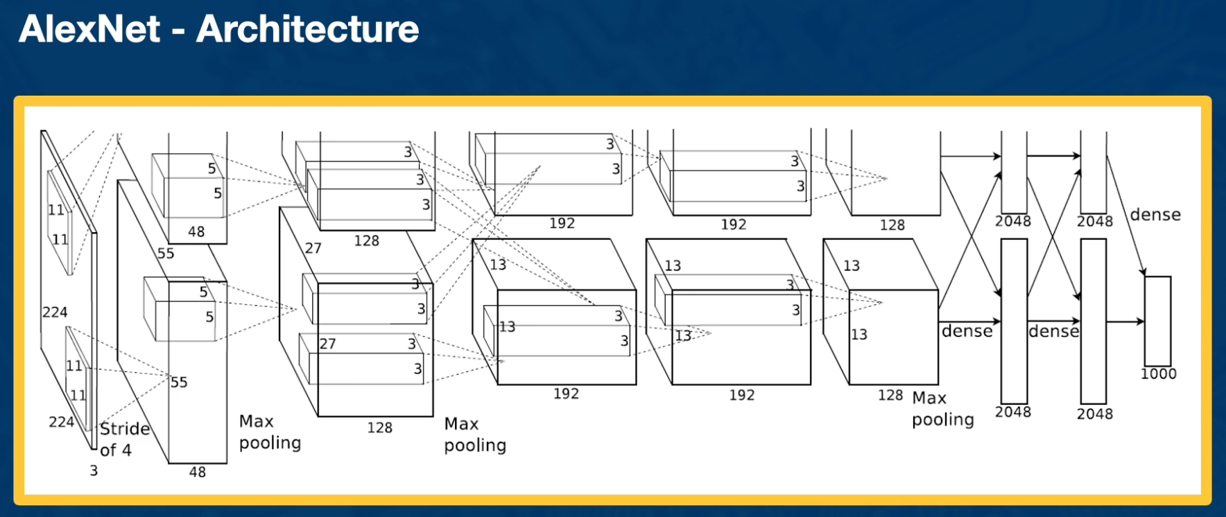
The first architecture that performed really well, is AlexNet.
Here we can see each layer laid out in terms of its dimensionality:
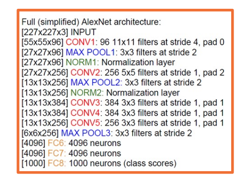
Key aspects:
- ReLU instead of sigmoid or tanh
- Specialized normalization layers
- PCA-based data augmentation
- Dropout
- Ensembling
VGG
VGG neural network that was very popular for a while.
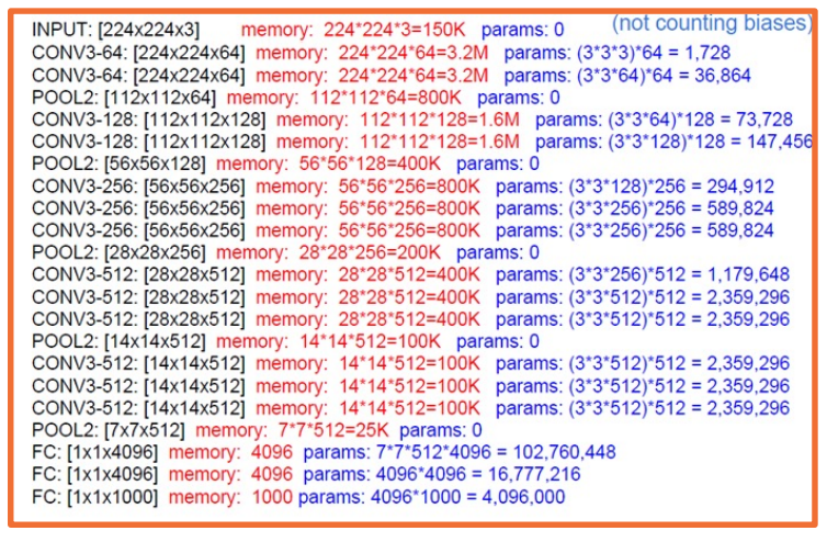
Key aspects:
- Repeated application of
- 3x3 conv (stride of 1, padding of 1)
- 2x2 max pooling (stride 2)
- Very large number of parameters
Most memory usage in convolution layers.
Inception
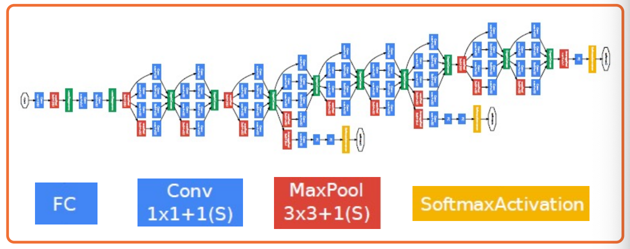
- Has repeated blocks that are repeated over and over again to form the neural networks.
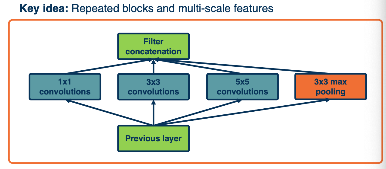
They have interesting aspects:
- They use parallel filters, that is, filters of different sizes in parallel.
- So that you can get features at multiple scales.
- Downsides is this increases computational complexity
The key idea here is we want to pick up complex features at multiple scales.
ResNet
Key idea: Allow information from a layer to propagate to any future layer (forward)
- Same is true for gradients!
Motivation behind resnet:
Eventually, as the depth of the neural networks increased, the ability to optimize them became a bottle neck. That is, as we increased the depth, we actually obtained higher error. So, researchers investigated why that was the case and it turns out that a simple modification you can make to these network architectures is to add a skip or residual connection.
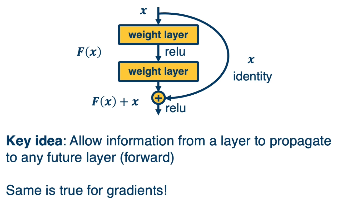
That is you can see here a path that goes from the in put x through some set of transformation, some weight layers and for example a relu and that transformation is added to the identity function. That is rather than having to output a completely new thing, given the input, you are just adding residual residual elements to the original input. You are just optimizing the weights such that you make small changes to the input rather than each layer having to output something completely new.
Evolving architecture and AutoML
- Evolutionary learning and reinforcement learning
- Prune over parameterized networks
- Learning of repeated blocks typical
Transfer Learning & Generalization
Generalization
Many types of errors can happen when training neural networks:
- Optimization error
- Even if your neural network can perfectly model the world, your optimization algorithm may not be able to find the good weights that model that function.
- Estimation error
- Even if we do find the best hypothesis, this best set of weights or parameters for our neural network that minimizes the training error, that does not mean necessarily that you will be able to generalize to the testing set.
- Modeling error
- Given a particular neural network architecture, your actual model that represents the real world may not be in that space. For example there may be no sets of weights that model the real world. (For example your model vs reality)
As models gets more complicated,
- Modeling error will decrease
- higher chance of predicting the real world with a complex model
- Estimation error will increase
- over fitting more and more
- Optimization error will increase
- dynamics of our optimization will get more difficult to handle.
Transfer learning
What if we do not have enough data?
- Step1: Train on large-scale dataset
- Step2: Take your custom data and initalize the network with weights trained in step 1
- Step3: Continue to train on new dataset
- Finetune: update all parameters
- Freeze feature layer: Update only last layer weights (used when not enough data)
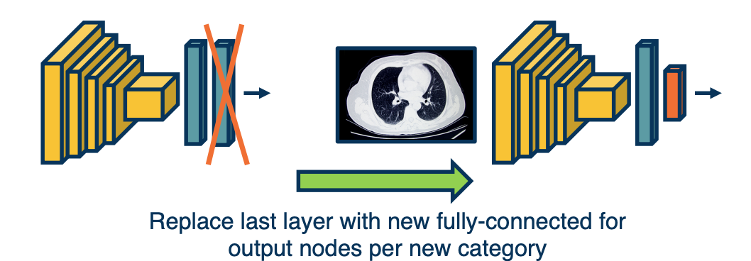
This works extremely well! Features learned for 1000 objects will also work well for 1001!. Generalizes even across tasks (classification to object detection).
But, his works well only if:
- If the source Dataset you train on is very different from the target dataset, transfer learning is not as effective
- If you have enough data for the target domain, it just results in faster convergence.
Effectiveness of more data
Another interesting finding is that we still have not reached a bottleneck in terms of amount of data, if we do have it. That is if we continue to add more and more data beyond the millions that we already have, performance continues to improve.
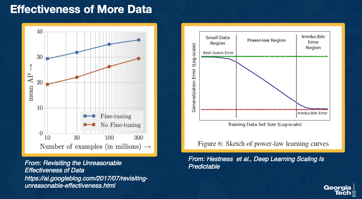
On the left, you can see that as we get to 300 million examples compared to the one million in image net, our performance on object detection as measured by a metric called mean average precision on the y axis continues to improve. You could see this both for fine tuning from image net classifier or weights to no fine tuning. In both cases you get significant improvement and the curve is still linear.
On the right, we can see some exploration where there is some irreducible error that we get to eventually, again in the log scale but this is for a particular domain. What is interesting is that there are different regimes that were identified. For example if you have too little data, then at some point, it is very difficult to decrease the error. Then you enter a power law region where essentially the training data set size in log scale continues to linearly improve the error again in log scale. And then again, at the end, you might get into some regime where you cannot reduce the error further.
Dealing with low labeled situations
Active research is still happening in terms of how far we can push in terms of reducing the number of labelled data. Unfortunately, in this field there is alot of different settings.
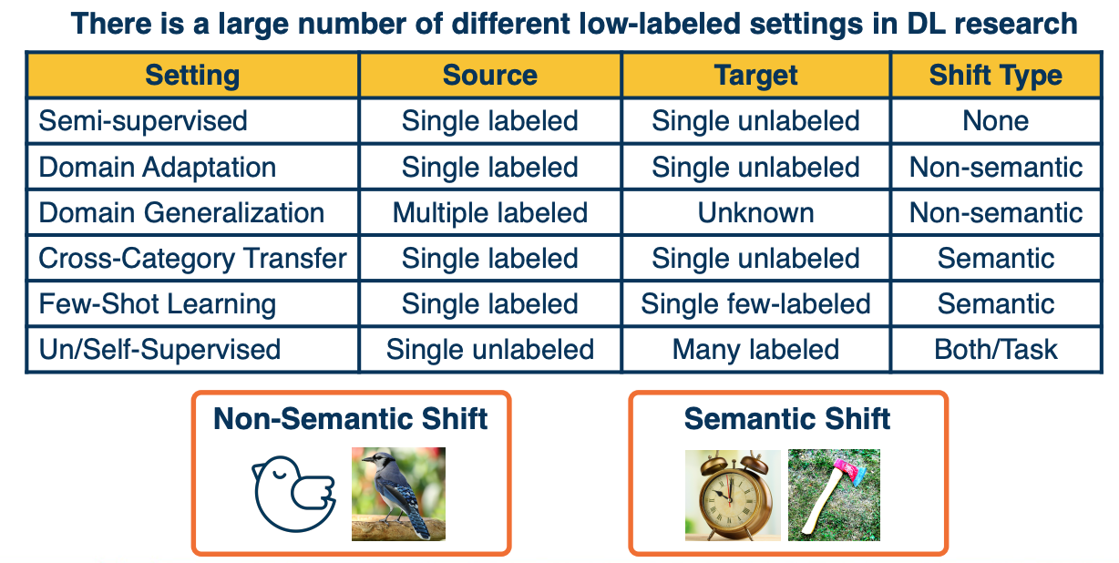
Lesson 7: Visualization
Readings
- Understanding Neural Networks Through Deep Visualization
- Grad-CAM: Visual Explanations from Deep Networks via Gradient-based Localization
Visualization of Neural Networks
Given a trained model, we like to understand what it learned. If you remember, all of the parameters of the neural network, both the convolution kernels as well as the fully connected layer weights, are all initialized to random values. After optimization, it should have found some set of good parameters that perform well on whatever task you trained it on.
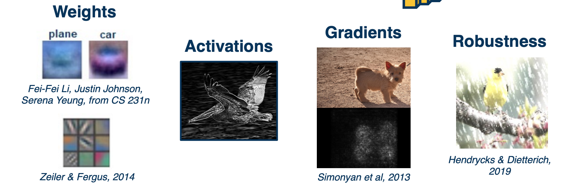
There are several ways to understand what is learned, even for simple linear classifiers. We have shown that we can take the learned weights, reshape them into images, and then plot them in a normalized way from zero to 255. This allows us to see rough templates of the objects, such as a car or a plane.
For convolution layers, we can actually do a little bit better. The convolution layers parameters are the kernel weights themselves, and so we can visualize what the kernels look like. Again these kernels are strided across an image, and high responses mean that the image patches have roughly similar types of features as the kernel. Here we see one example where linear features such as different oriented edges are learned.
We can also plot the activations after running a kernel across an image, you get an output/feature/activation map. These activation maps represent spatial locations with high values that are highly correlated with the kernel - we can plot them in a visual manner and try to understand what kind of features the neural network has learned.
We can do more interesting things, gradients are the key bread and butter of deep neural networks. These are what is used to optimize the networks themselves. Using gradients or gradient statistics, will allow us to better understand what the network is learning.
Finally, we can test various aspects of robustness for neural networks. For example we can try to see what are the weaknesses or biases of the neural network and use that to improve the performance.
For fully connected layers, if the nodes are connected to the image itself, then you can actually just take the weights, and reshape them into the images. Since you have one weight per pixel, we know that the number of weights should be equivalent to the number of pixels, and we can reshape it and scale the values between zero to 255 which are valid pixel images. We can then visualize the results and you will see various rough templates for each of the objects. For example for a car, you can roughly see the bottom of the car which tends to have dark pixels. The hood which have reflections, the windows which have darker pixels again and so on. However if you have a complicated CNN, the fully connected layers at the end are not connected to the pixels. They are connected to output or feature maps from the last convolution layer - so you cannot visualize them as easily.
Problem:
- 3x3 filters and small conv outputs are hard to interpret.
Theres a link build by other students in gatech to visualize cnn found here.
Dimensionality Reduction: t-SNE
We can also take the activations of any layer (FC, conv) and perform dimensionality reduction and convert them into vectors.
- Often reduce to two dimensions for plotting
- Can also use PCA
- or t-SNE
- Performs non linear mapping to preserve pair-wise distances.
- Features vectors that are very similar according to some distance metric are shown together here in the two dimensional plot whereas feature vectors that are very different will end up very far apart.
The above visualization is for the MNIST example where you have digits from 0 to 9, we can plot the different points in the two dimensions according to their categories based on their color. What you can see is they are pretty well separated after training - probably means we are able to learn a really good classifier.
Summary and Caveats
While these methods provide some visually interpretable representations, they can be misleading or uninformative.
Assessing interpretability is difficult
- Requires user studies to show usefulness
- E.g. they allow a user to predict mistakes beforehand
Neural networks learn distributed representation
- (no one node represents a particular feature)
- This makes interpretation difficult
Gradient-Based Visualizations
Backward pass gives us Gradients for all the layer that is the gradient of the loss with respect to that particular layer. This shows us how the loss changes as we perform small perturbations on those layers. While during optimization, we have only computed this for all the layers in the neural network, we can also do it with respect to the input as well.
In other words, if we make small pixel changes in the image, how does the loss change? This can be useful not just for optimization but also to understand what was learned.
- Gradient of loss with respect to all layers (including input)
- This allows us to understand the sensitivity of those particular features with respect to the loss function.
- Gradient of any layer with respect to input (by cutting off computation graph)
Gradient of loss w.r.t Image
Idea: We can back propagate all the way to the image.
- Gives us some information about the sensitivity of the loss to individual pixel changes.
- Large sensitivity that is larger gradients implies important pixels
- Because if we change these pixels in small ways, then it causes a change in the loss function
- These are often called Saliency Maps
- Because it shows us what we think the neural network might find important in the input.
In practice:
- Instead of finding the partial derivative of the loss with respect to the input, we will actually find the partial derivative of the classifier scored before the softmax with respect to the input.
- Why might this be the case?
- Applying the softmax function and then the loss function actually adds some complexity. For example the neural network can actually reduce the scores of the other classes in order to increase the scores of the correct class after softmax. So this might introduce some weird effects in terms of the gradient.
- Why might this be the case?
- Take the absolute value of the gradient.
- We do not care which direction the loss function changes, all we care about is that the loss changes.
- We can also sum across all of the channels as well.
- So we do not care that a particular red channel in the image has this effect. What we care about is one particular pixel that represents parts of objects.
Object segmentation for Free!
We can actually take the gradients and visualize them across the image as shown here, where darker values are smaller gradients and lighter values are larger gradient.
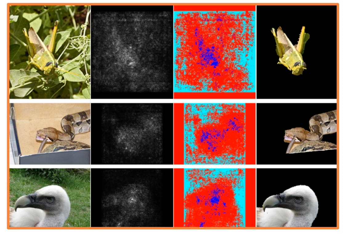
What we will find is that higher gradients tend to corresponds to parts of the object that we are trying to classify. So we can actually apply traditional computer vision segmentation algorithms and try to find regions within this gradient image of values that are similar. (Try to group similar values together). When we apply this, we can actually get a segmentation mask of the object - we obtain which pixels in the image actually the object or correspond to the object.
This is a little surprising because during our supervision, we never gave it the segmentation masks. All we gave it was there is a particular type of object in this image, and out of that we actually get object segmentation for free, which is surprising because it is not part of supervision.
Detecting Bias
We can use this to debug various issues, such as detect dataset bias. For example snow used to misclassify as wolf.
- Incorrect predictions are also informative!
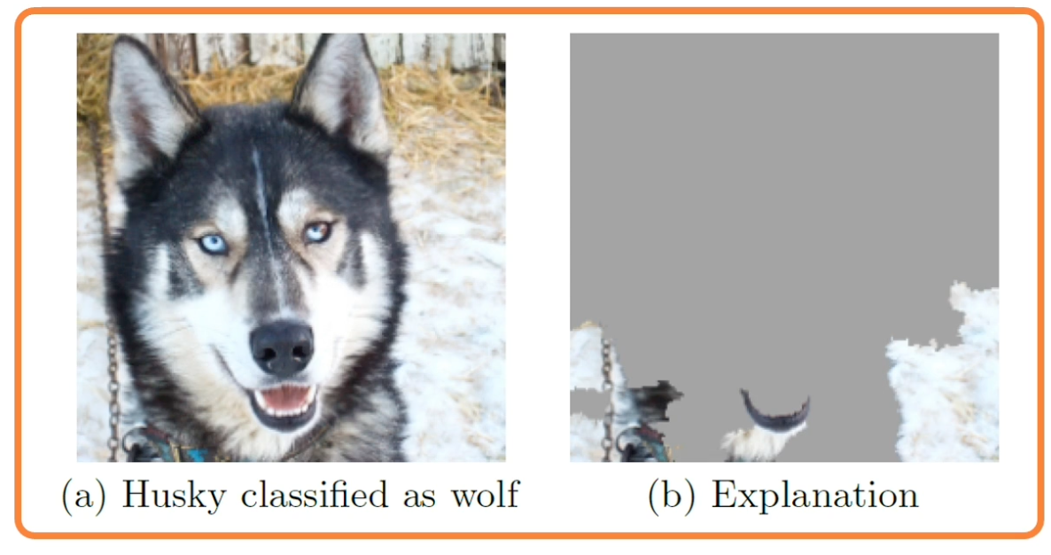 The wolf white skin is detected as snow
In the above example, the neural network just learn to classify the object based on the background, and when we plot the gradients, we see that the gradients and segmentation that results really focus on the snow, rather than an object we care about.
Gradient of Activation with respect to Input
Rather than the derivative of the loss with respect to the input, we can also find the partial derivative of some random activation that we choose (at random) inside the network with respect to the input. We can run forward function only up until that layer and when we run backpropagation, we will actually get the gradient of this particular activation with respect to the input. This is the magic of back propagation and gradient descent across an arbitrary computation graph.
Steps:
- Pick a neuron
- Find gradient of its activation w.r.t. input image
- Can first find highest activated image patches using its corresponding neuron (based on receptive field)
Guided Backprop
Now, the way we backpropagate gradient is obviously the right way to do it for things like optimization gradient but may not actually be the best for things like visualization.
For example, for visualization, we do not really necessarily care about negative influence. That is, you might have parts of an image that decrease feature activation and so when we find the gradients of the feature activations with respect to the image, we will get negative gradients
- But there is probably many parts of the image that if perturbed will decrease particular features.
So we may not want to visualize this aspect, we may only want positive influence visualized. So there is alot of different methods such as guided backprop that tried to approve this. Here is a visual depiction:
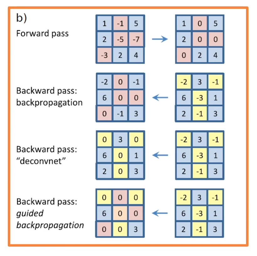
- On the top, you can see the forward pass. This is through a ReLU.
- You can see that the negative values are zeroed out while the positive values are just passed as is.
- When you do a backwards pass for the values that were negative in the input, you zeroed out those gradients.
However, you can also change this a little bit by what is called a deconvnet.
Rather than just pass back the gradients as we described, we will take the gradients and only pass back the positive gradient. In other words we will remove the negative gradients (in yellow boxes) or negative influence because we may not want to visualize them. This changes the way we do backpropagation so we do what is called the guided backpropagation which combines both of these ideas (orange and yellow boxes).
- Zero out both the forward pass and negative backwards gradient.
- So only positive influences will be propagated.
Here we see some examples of guided backpopgation:
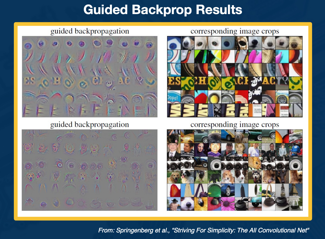
First find the maximally activated patches as we described - find image patches that really activate particular features or kernels in the neural network that we care about. We can then visualize the gradients of the activations with respect to the input.
We can see is a much nicer, clear results that really focus on the objects or the interesting parts of the image themselves. You can also see on the bottom when you do this for deeper parts of the network as you get larger receptive fields.
So now let’s use these methods to visualize the features that we learn across the different parrts of a network. We will take VGG as an example and perform layer by layer visualizations.
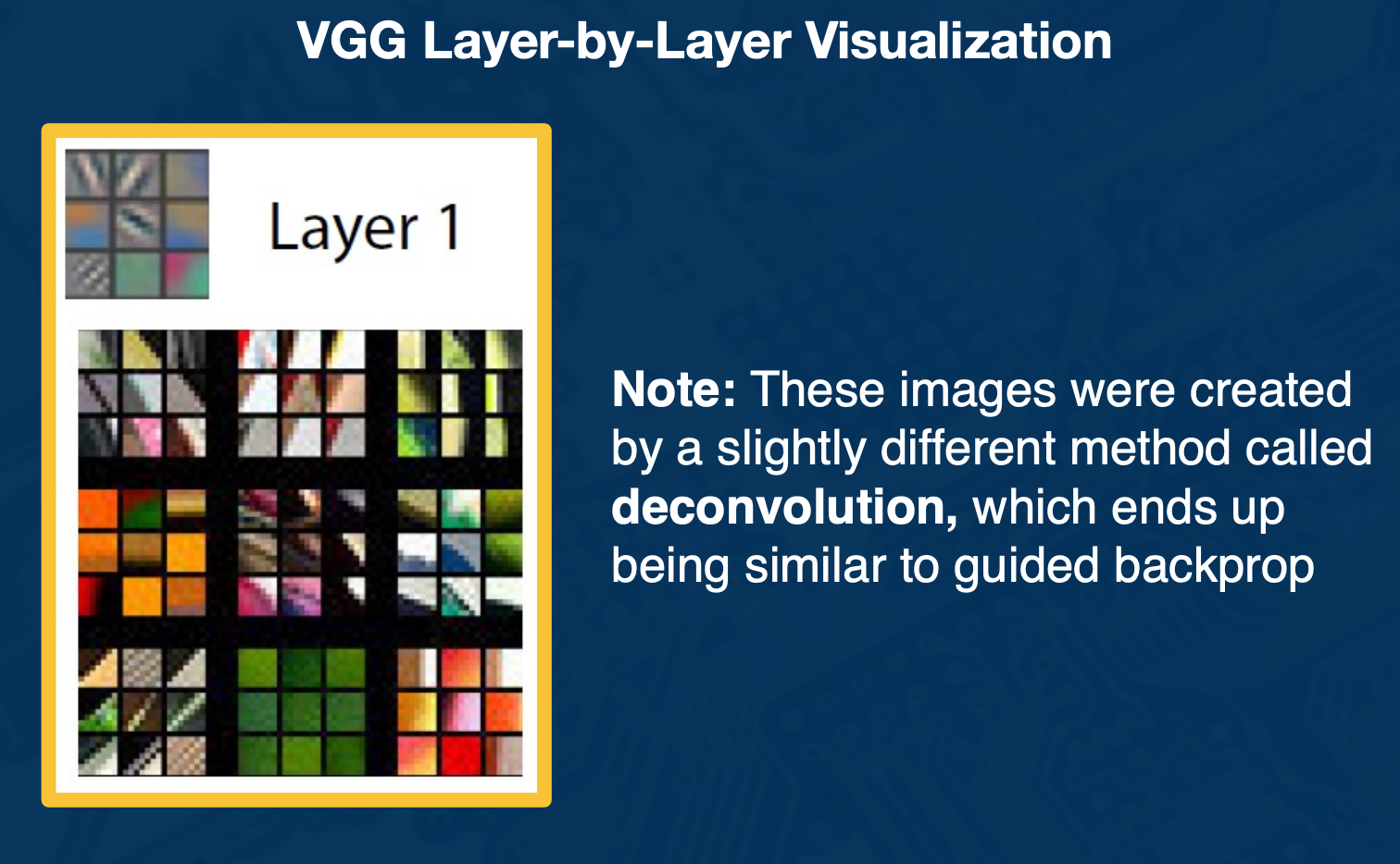
Here we can see that layer one in the neural network learns very low level features such as edge orientation. Sometimes it also learn things like color or texture patterns such as repeated dots.
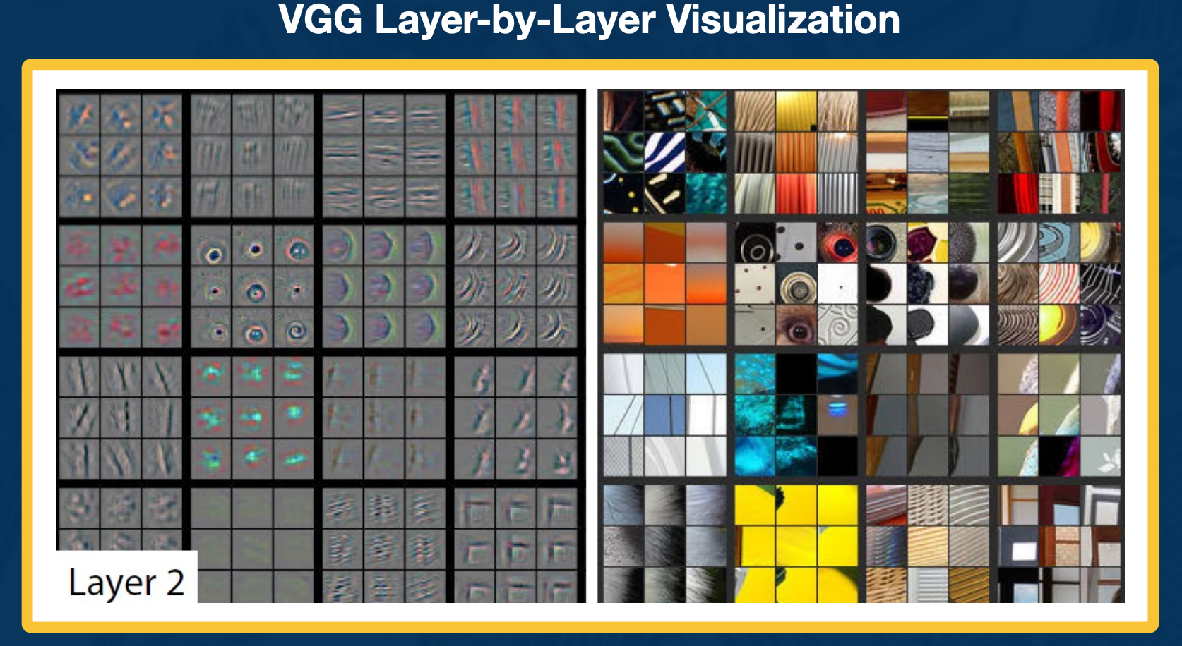
In layer two, we see that actually these low level features such as edges are combined in order to find higher level features such as motifs. We also have more interesting color, texture or pattern.
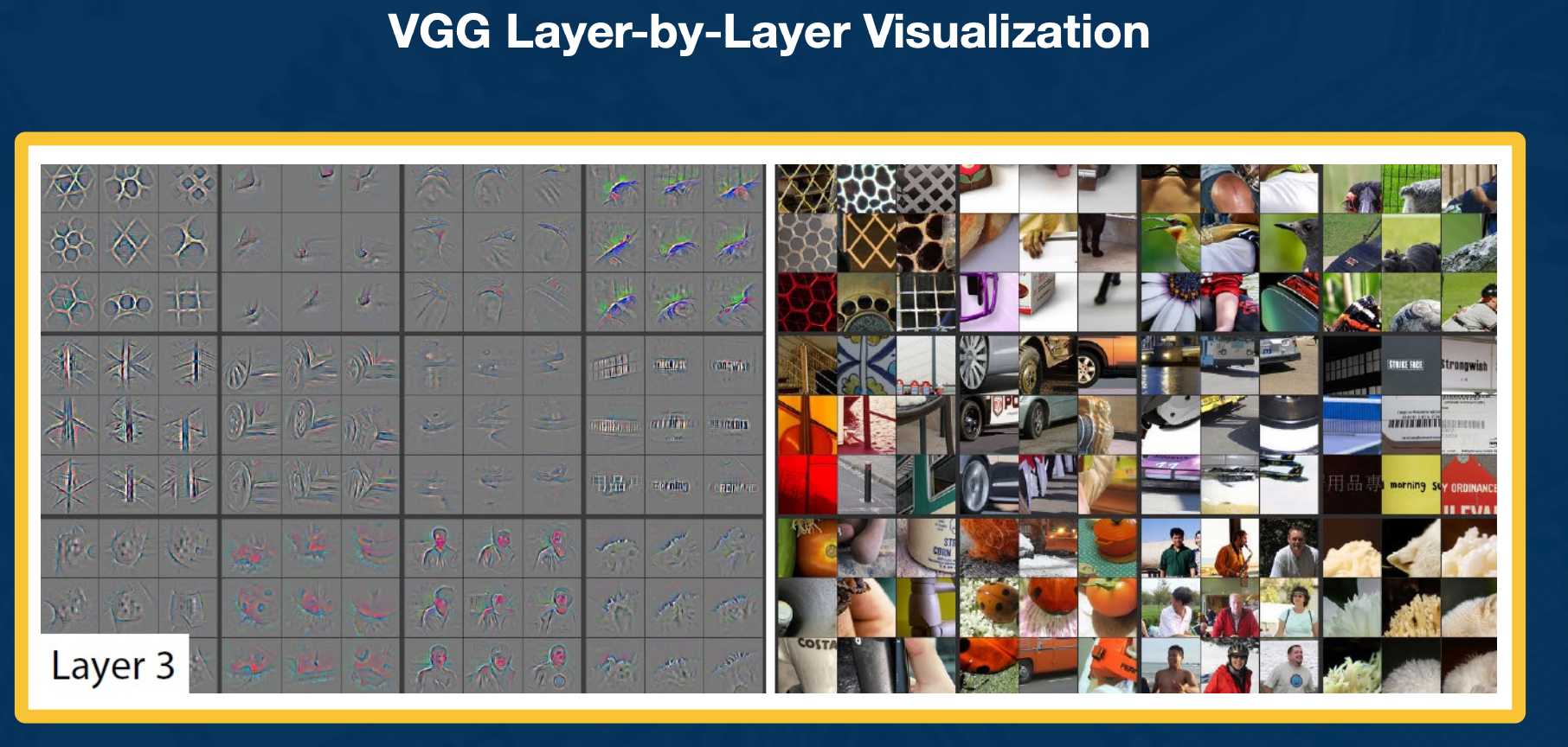
In layer three, we get even more high level and abstract, we find things like wheels of a car or different parts of people.
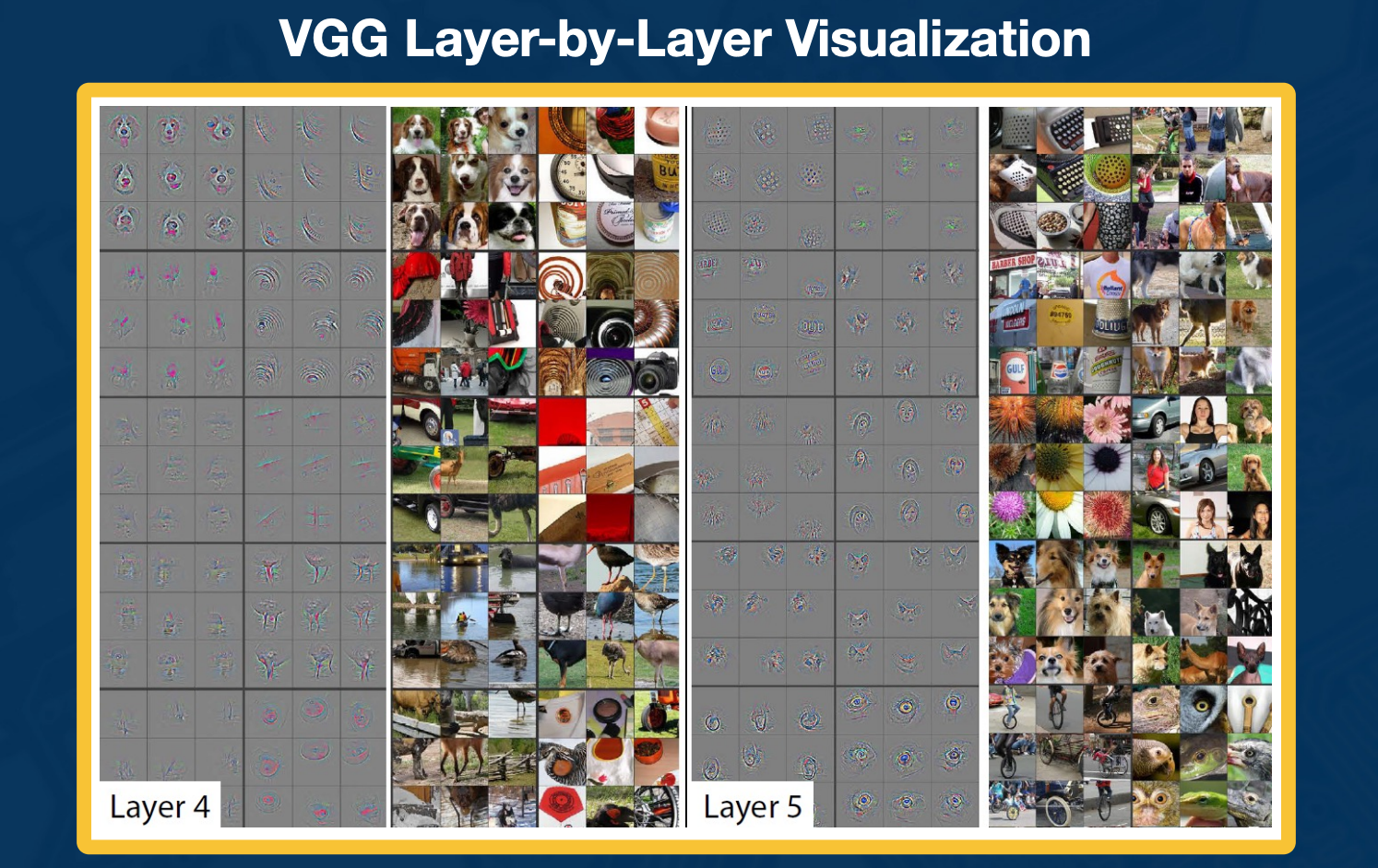
Finally, in very deep convolution layers, it is actually finding entire object parts or entire objects themselves.
Grad-CAM
As researchers began plotting saliency maps, more and more sophisticated methods were developed to understand what the neural network considers important. Here is one such method called Grad-CAM:
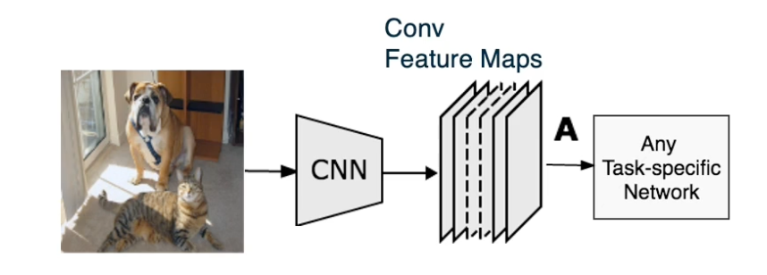
Given an image, we can feed it through a convolution neural network. We will take the feature maps of the last convolution layer. We do this because we think that the feature maps at end of the network will have more abstract or high level features that are important. We can then have task specific networks such as fully connected layers for image classification.
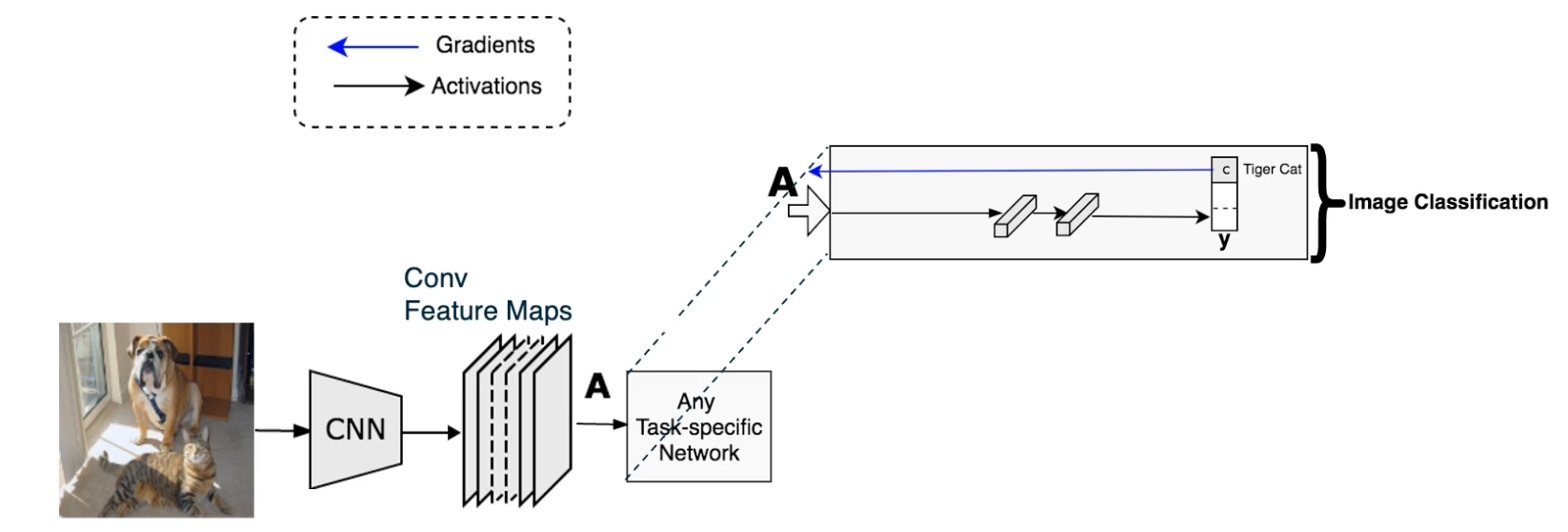
Given a particular class C, we can then back propagate to get the partial derivative of the class output that is the class score. We don’t use probability with respect to the feature maps that care about. So we only backpropagate to the feature maps that we want.
This results in a set of gradients in a set of gradients in the same shape as feature maps. If you remember in the feature maps, each channel corresponds to a particular kernel or filter. We try to weight them to find particular important channels as represented by high gradients and we will assign higher weights to those channels. Specifically we will use methods similar to attention mechanisms (that will learn later in the class). We will have a per channel waiting that is represented here as alpha.
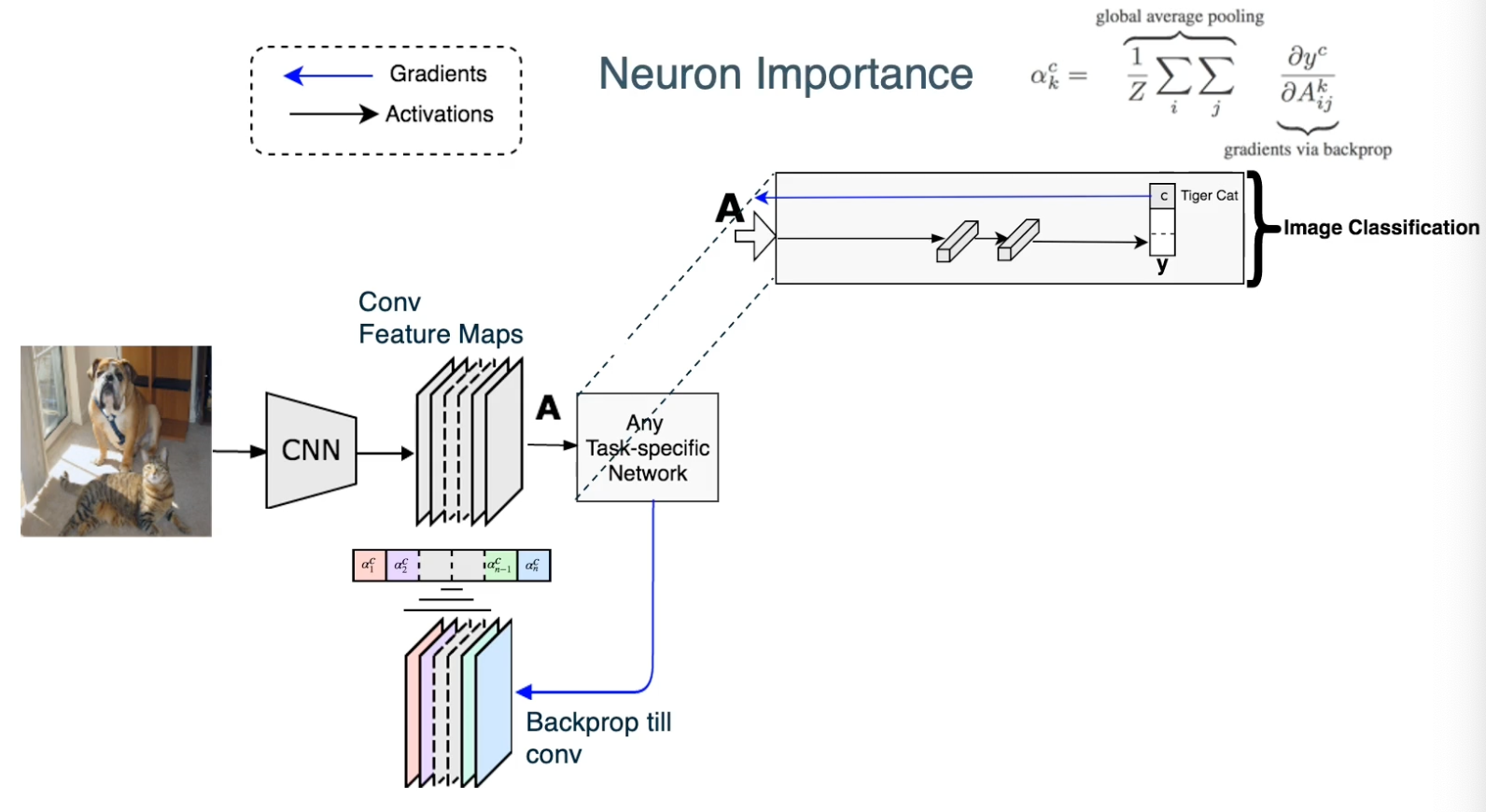
The way we will compute this is very simple, we will just do a global average pooling for each channel of the gradients. In other words, for each channel, we will sum up all the gradients across the channel of the gradients of the score with respect to the activations and normalize it. This results for each channel K a particular weighting.
We will multiply the forward activations the feature maps by this weighting. So each channel will be multiplied by its corresponding weight.
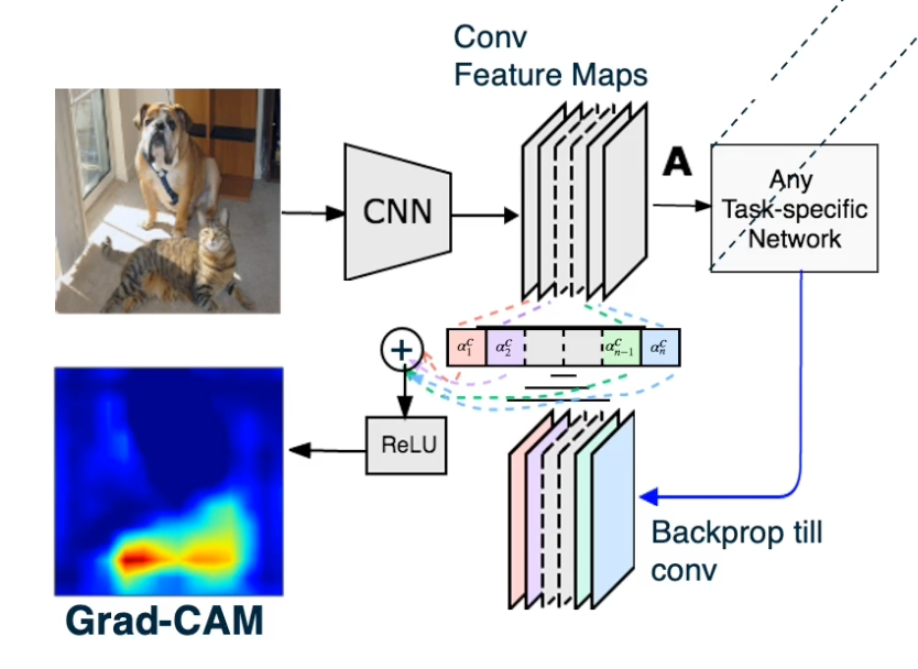
We will also feed a ReLU activation function because we only care about positive features. This will result in this particular output where values that are important as represented by high gradients or channels that have high gradient will have higher values here.
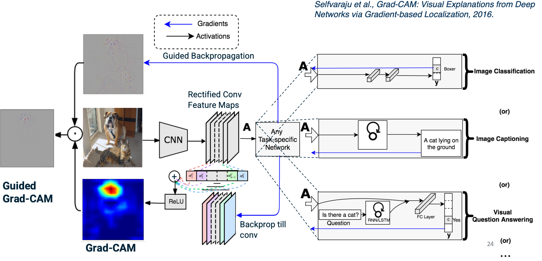
Note that this is not a method that specific to what the task is. We can calculate this for any task. And so what we actually also do is combine this grad cam output, which essentially is the feature maps weighted by their importance as represented by high gradients by the guided backpropagation output.
So guided backpropagation as we discussed will result in again this output representing the gradients. When we multiply these together element wise, we will be doing is we are emphasizing parts of the guided backpropagation that are important - will reemphasize parts that corresponds to things like objects that are highly representative or affect the loss function greatly. This is called guided Grad-CAM.
Here are some example outputs:
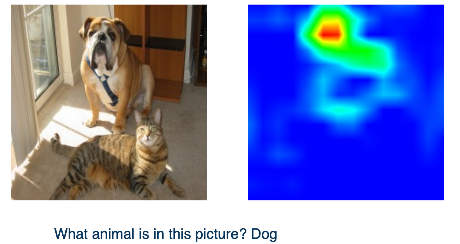
When the answer for the NN is a dog, the Grad-CAM shows the dog in the image.
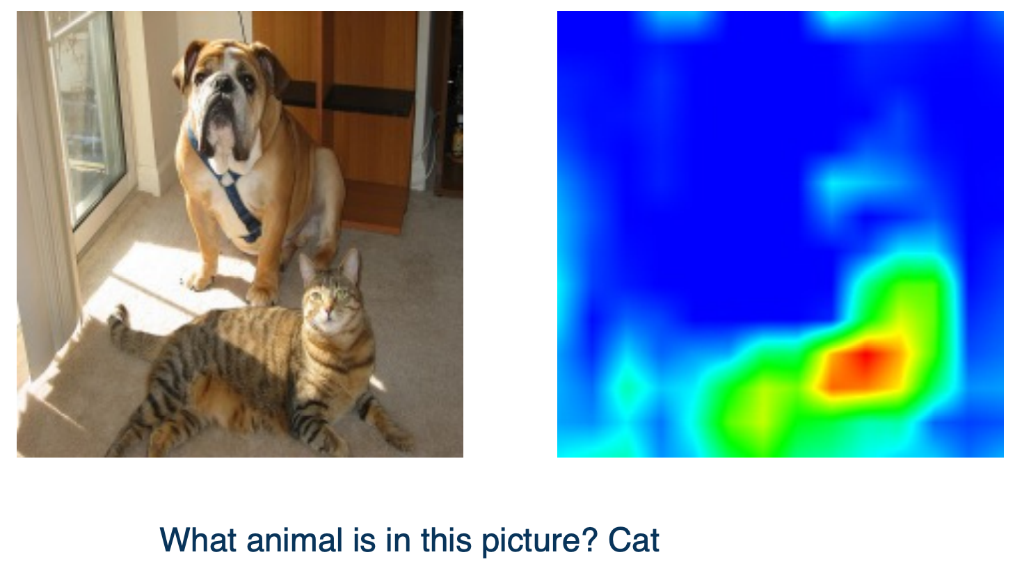
But if the NN output cat since there are multiple animals in the picture, the Grad-CAM will emphasize the cat.
So in summary,
- Gradients are important not just for optimization, but also for analyzing what neural networks have learned
- Standard backprop not always the most informative for visualization purposes
- Several ways to modify the gradient flow to improve visualization results
Optimizing the Input Images
We can also optimize the image itself and get some interesting results.
The key idea here is since we have already the gradients of the scores with respect to the inputs, can we optimize the image itself to maximize the score?
- We can perform gradient descent (or ascent) and modify the image using these gradients.
Why?
- We can generate images from scratch.
- Start with a random image, apply the gradients over and over again, and actually generate interesting looking images.
- Adversarial examples
- We can also start with a real image and apply the gradient.
- We can actually do this for the score of the class that is not in the image.
- For example, we can choose elephant in this particular image and we can actually optimize the image in order to maximize this particular class.
- It turns out that we can make a small number of modification to really fool the network. In the sense that the image will still look like a dog to humans, but with respect to the network it will confidently say that it is an elephant.
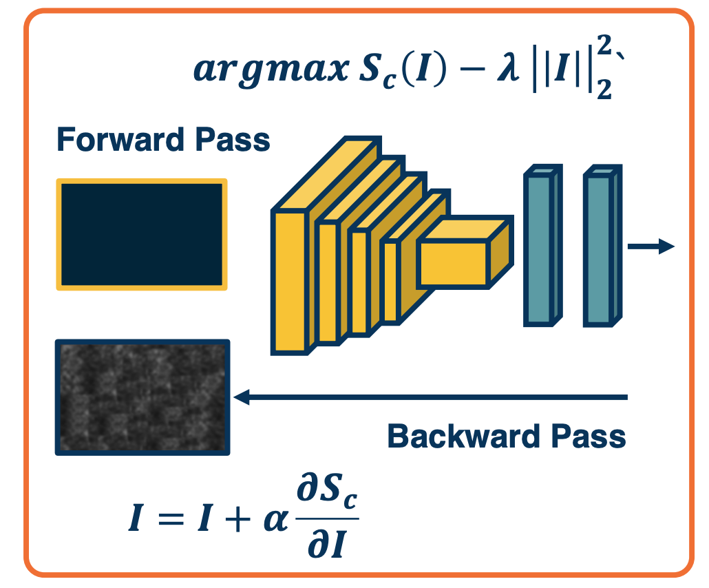
Gradient Ascent on the Scores
We can do this by performing Gradient ascent on the image. We can compute the gradient of the score for a particular class that we care about with respect to the input image.
Rather than subtracting the learning rate times the gradient, we will add the learning rate times the gradient. This has the effect of maximizing the score.
We can also have a regularization term ($-\lambda \lvert\lvert I \lvert\lvert^2$) - for example preferring smaller pixel values. Note that we are subtracting the regularization because we are performing ascent.
The full procedure:
- Start from a random/zero image, compute the forward pass, gradients, perform ascent and then iterate.
- Note that we are using scores here so that we do not minimize other class scores after we compute softmax probabilities.
- Here because we are using the raw scores themselves, the network is forced to directly increase the score for the class that we care about.
Often we need some form of regularization to induce statistics of natural imagery
- e.g small pixel values, spatial smoothness.
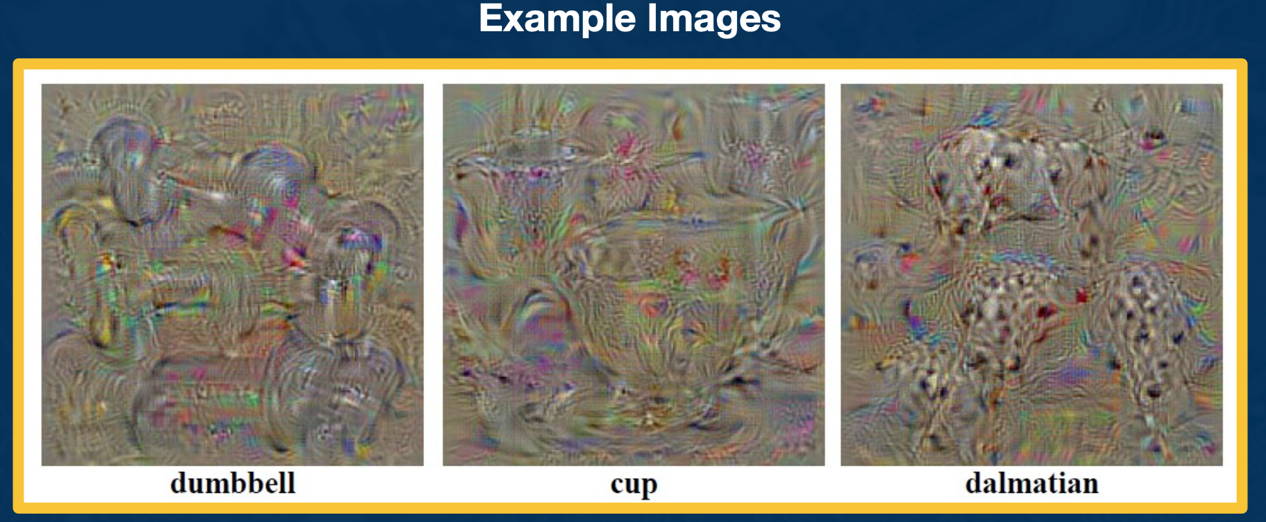
You can observe that the particular objects that we wanted to maximize the score of appears in many different locations across the generated image, but it is cool that we can automatically generate images from scratch.
We can improve the results with various tricks:
- Perform clipping of small values and gradients.
- Can apply Gaussian blurring at various points in time across this optimization.
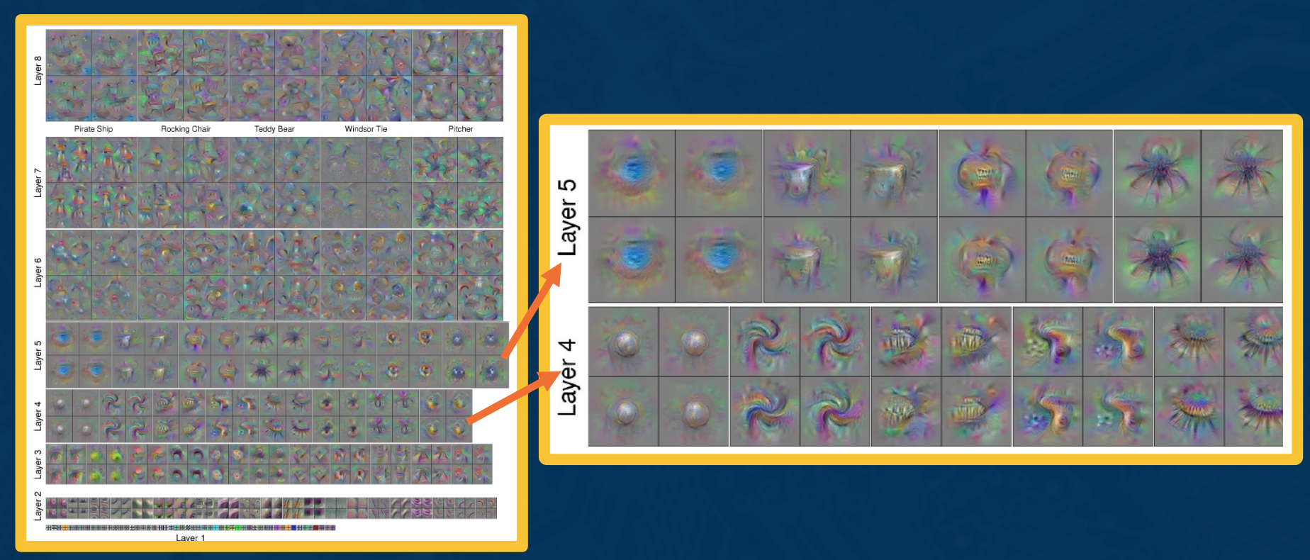
We can do this across the entire neural network - does not have to be maximizing particular output scores, we can maximize any activation anywhere in the neural network and try to see what are the images that maximize this.
Here, we can see the particular types of features that the filters or kernels might be representing.
In summary,
- We can optimize the input image to generate examples to increase class scores or activations
- This can show us a great deal about what examples (not in the training set) activate the network
Testing Robustness
We will now focus on testing the robustness of neural networks to particular things like perturbation.
- We will also show how to generate adversarial images by optimizing the input.
Gradient Ascent on the Scores Gone Wrong!
Rather than starting from zero image, what if we start from a real image? What if, in addition we optimize the score of an arbitrary incorrect class?
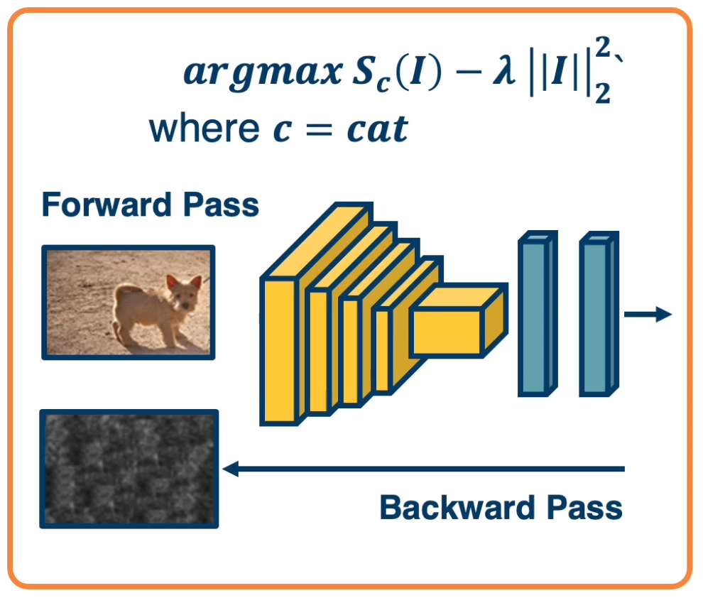 The image is a dog but we want to optimize for a cat
Surprising result: You need very small amount of pixel changes to make the network confidently Wrong!
Example of Adversarial Noise
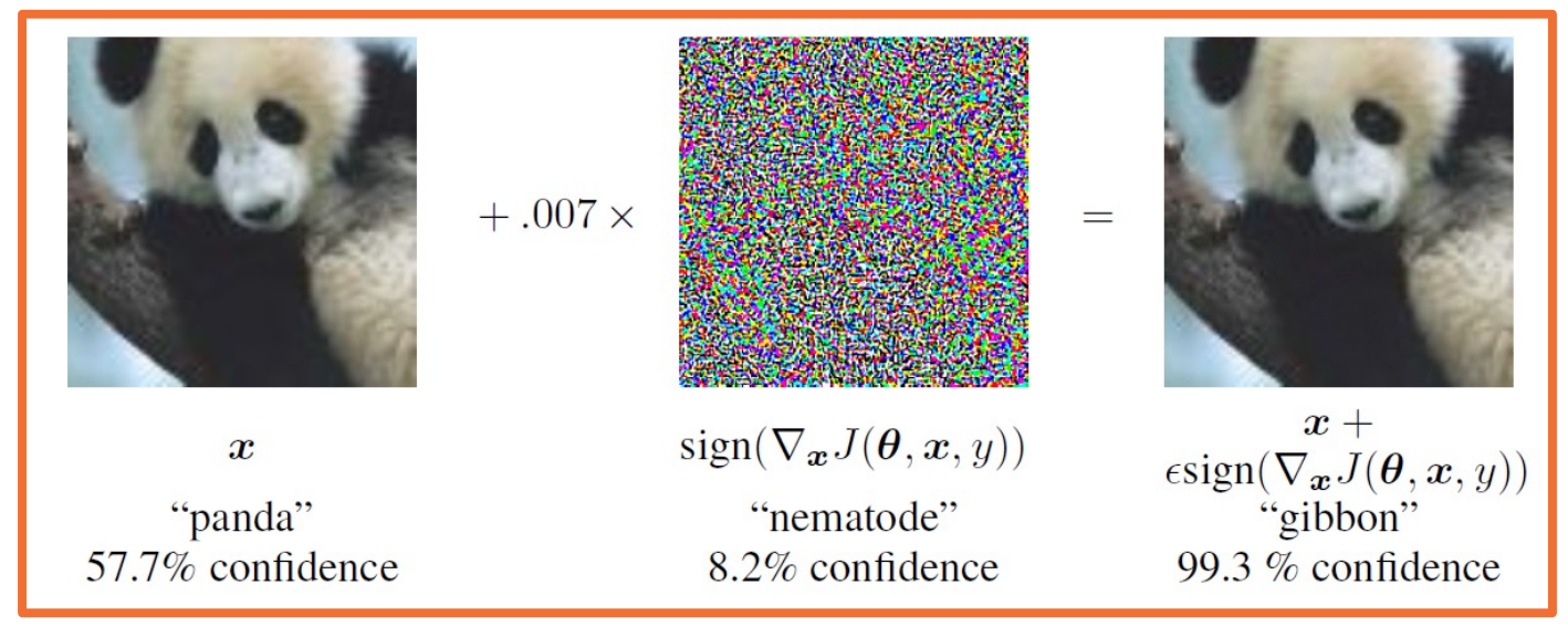
Here is an example of the perturbation that we can apply to make it confidently wrong - by adding the random noise and the network thinks with 99% confidence whereas to a human the image looks completely the same.
Note, this problem is not specific to deep learning!
- Other methods also suffer from it
- Can show how linearity (even at the end) are susceptible to this as well.
- For example, you can think about adding across a high dimensional set of values very small values per dimension such at the end when you add up the weighted summation, it actually ends up the wrong class.
Variation of attacks
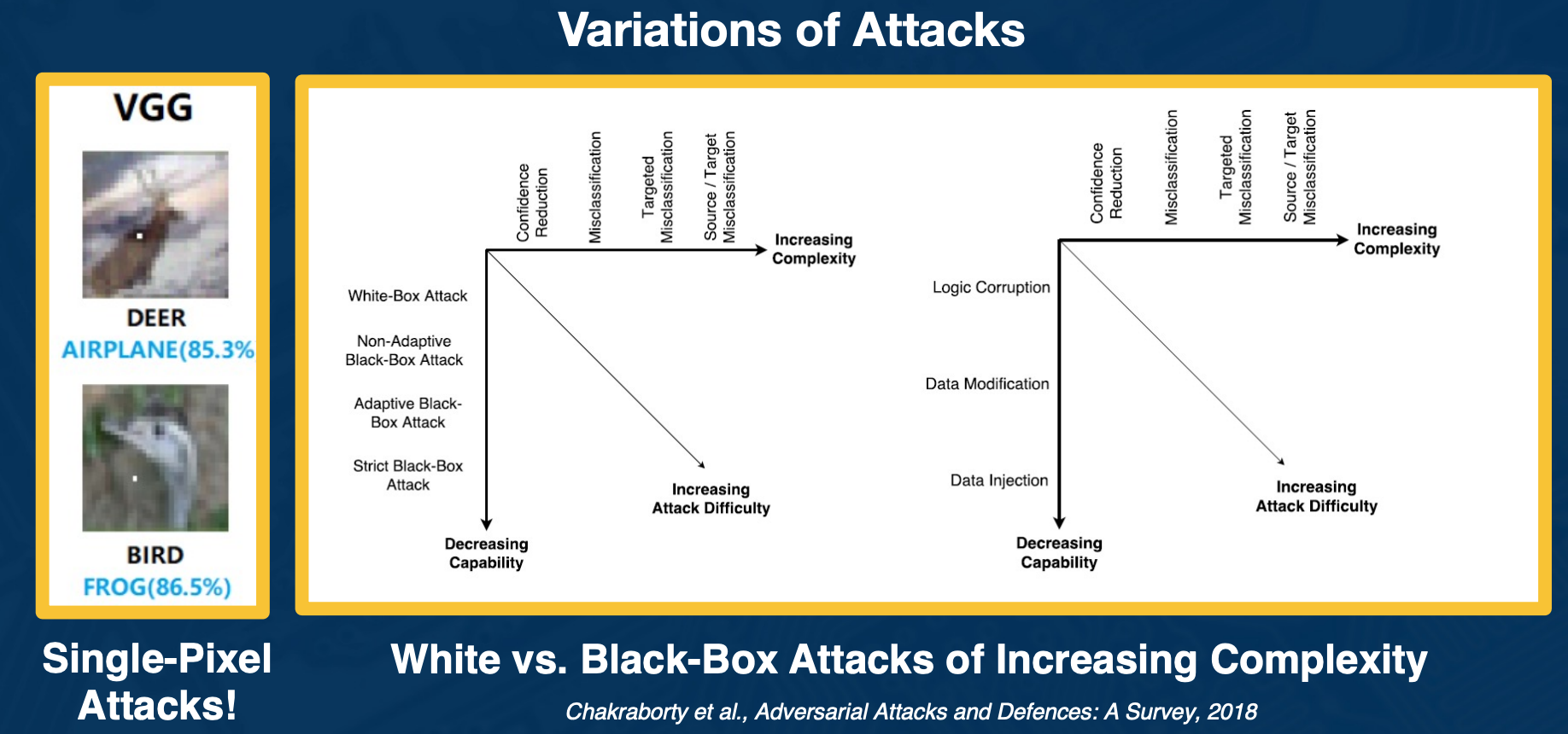
There is actually a range of attacks you can apply to attack deep learning. For example, researchers have shown that actually you can have single pixel attacks where literally you change one pixel in a ay to make the neural network wrong.
There is also a range of types of information that you might or might not have available as an attacker. For example the method that we have talked about requires performing gradient ascent on the image using neural network. Clearly you have to know the architecture and the learned weights in order to do this.
There are other black-box attacks where maybe all you can see are the predictions of the neural network and you can still try to generate or find images that fool it. There is also methods that poison the training data set and so on.
Similar to other security-related areas, it’s an active cat-and-mouse game
Several defenses such as:
- Training with adversarial examples
- Perturbations, noise, or reencoding of inputs
- therefore perturbations that have been found to work are no longer as effective.
There are not universal methods that are robust to all types of attacks. Unfortunately we still do not know how to make NN robust across all these types of attacks.
Other forms of robustness testing
We can also see how different types of perturbations affects performance and we can see this for different types of architectures.
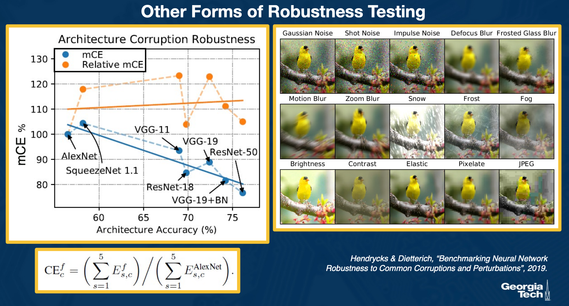
On the left you see a specialized corruption error metric that sums up the contributions across all the different types of corruption and shows this in a relative and non relative manner for many different types of architectures. The key point here is that the relative mean corruption error is actually relatively flat or slightly increasing, meaning that some of the architectures such as ResNet perform much better overall, but maybe are not as improved in terms of corruption.
Shape vs Texture Bias
We can also try to understand the biases of CNN.
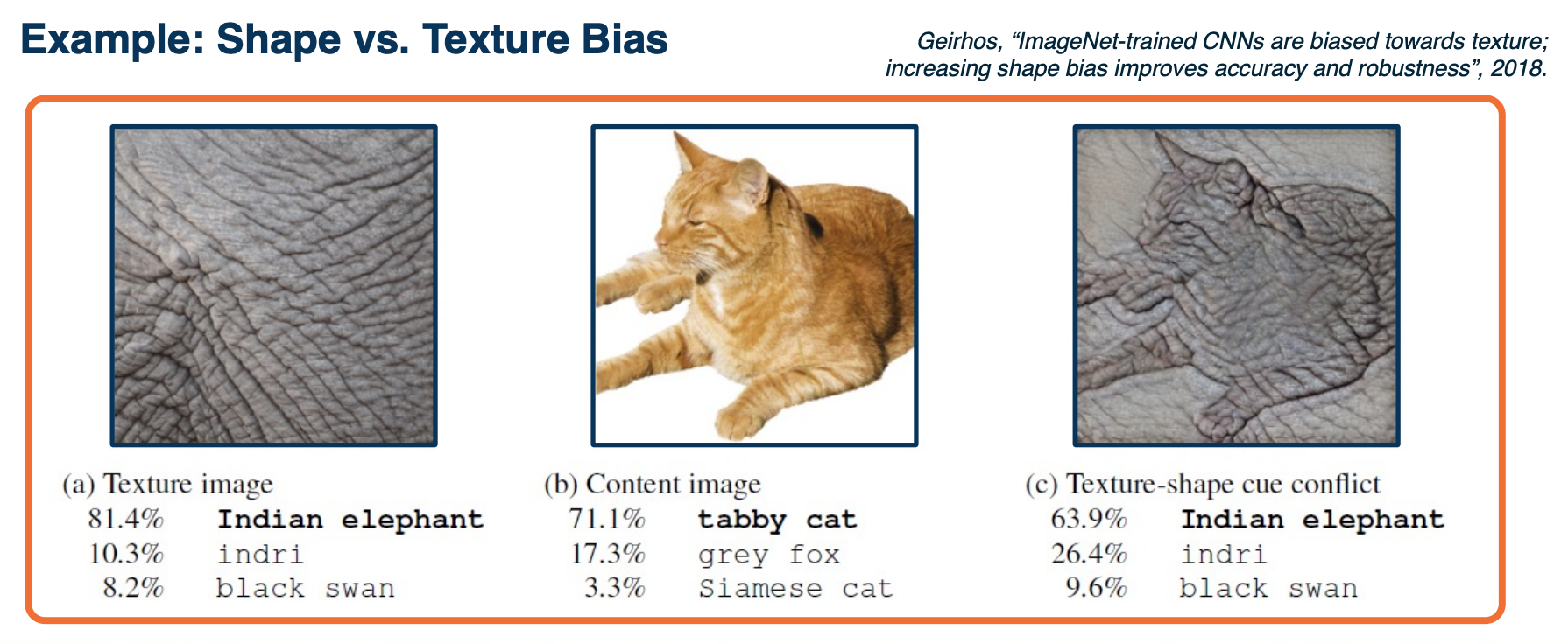
An example of this is the shape and texture bias. We can take an image of a cat but change the texture to an elephant and humans will inevitability say that this is a cat.
- However, CNN are much more bias toward saying that it is an elephant.
- meaning that they weigh more heavily towards texture and shapes.
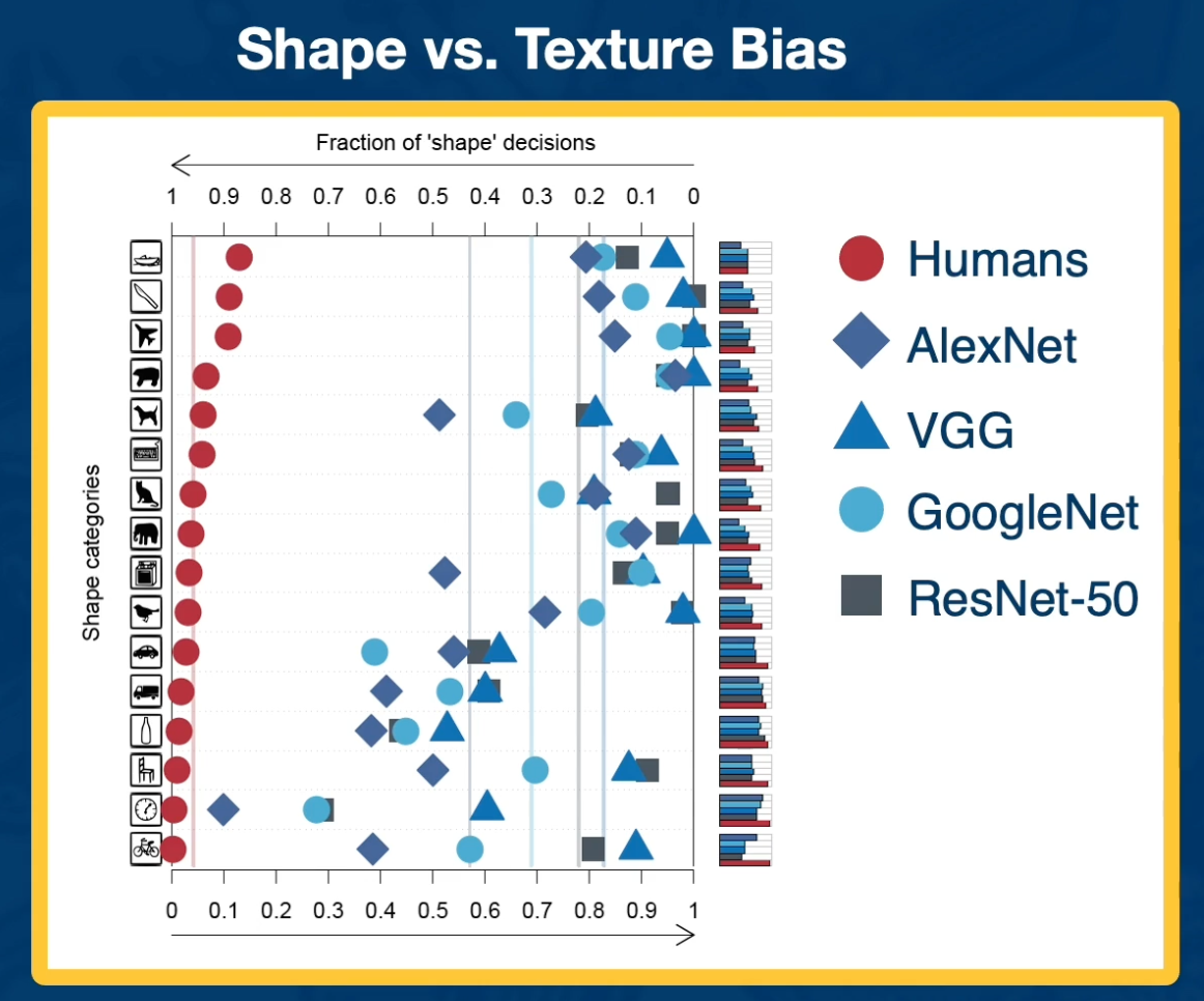
Something interesting is that all the NN are biased towards texture especially the ones that are much more effective such as ResNet are much more heavily bias towards textures compared to things like AlexNet which does not perform as well but have a much s tronger shape.
In Summary,
- Various ways to test the robustness and biases of neural networks
- Adversarial examples have implications for understanding and trusting them
- Exploring the gain of different architectures in terms of robustness and biases can also be used to understand what has been learned
Style Transfer
Style transfer - Generate images that match the content of one particular image (based on the content) but also maintaining the overall style or texture of a style image.
We can generate images through backpropagation. We can just forward pass through the network and then compute the gradients in the backward pass and apply those gradients.
- Can apply regularization to ensure that we match image statistics.
But what if we want to preserve the content of some specific image during this generation process? One idea that we will be using is matching the features of different layers across the forward pass of this generated image as well as some content image that we want to replicate. We can also have a loss function for this in order to improve the generation.
Matching Features to Replicate Content
We have an image, lets say of a dog that we want to replicate. We will feed that image through a CNN to extract the forward activations or the feature values across all the layers. We will then do for the image generation what we did before, we will take an image, let’s say a zero image or a random image and also feed it through the convolutional neural network - and then we will try to have a loss that optimizes the image to minimize the difference between the features for the generated image and the features for the content image that we care about.
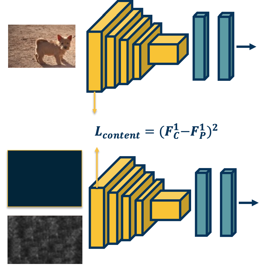
Here, we are showing the first layer, let’s say we extract FC which is the content features for layer 1 and then we will subtract it from the features of the generated image at layer 1. We will use that loss to back propagate - we will update the actual image, compute the gradients of this loss w.r.t to the image apply those gradients to the image.
If we are doing gradient descent, we are going to try to reduce this loss (minimize the difference in the feature space).
Multiple Content Losses
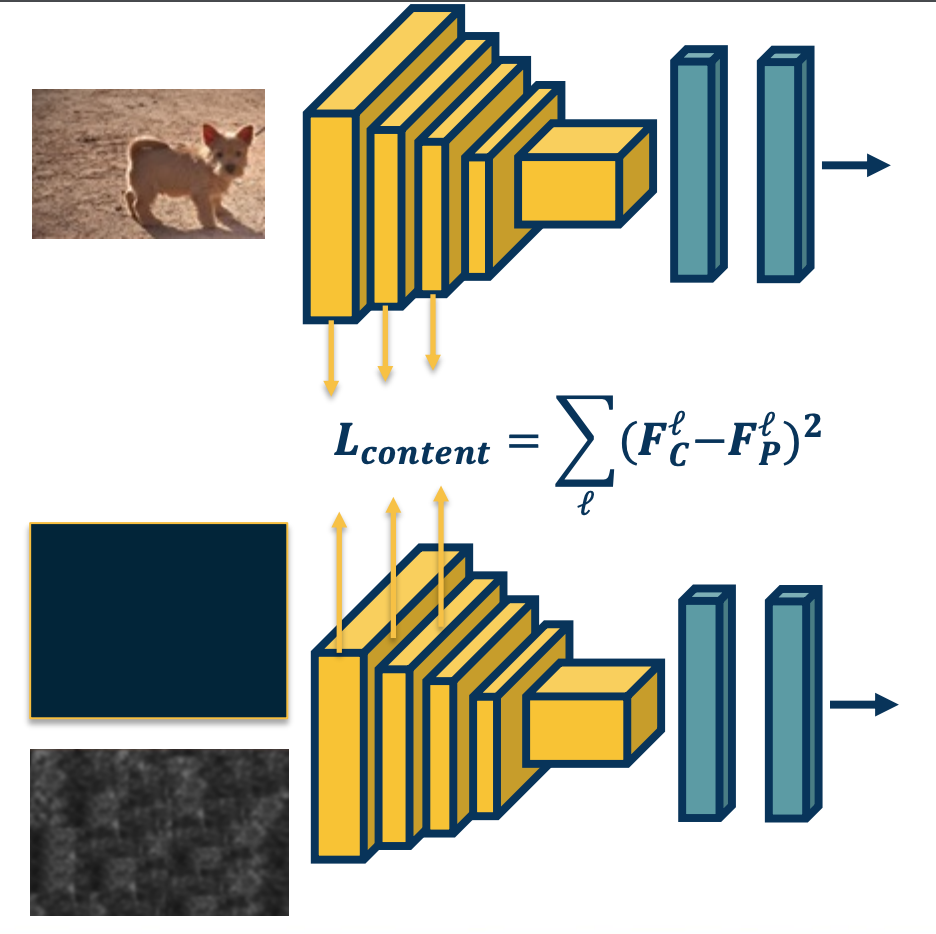
We can actually do this for many different layers - We just sum up the losses.
Because this is in a computation graph, when there are multiple backwards edges coming to the same node then you sum up the losses. Tus, we can just perform this loss function across all the different layers or whatever layers we choose and perform gradient descent. In other words, optimize or generate an image that minimizes this loss - thereby matching the image content and features across the entire neural network.
Replicating Content and Style
What if we want to perform the same optimization - except that we want a content of one image and texture of another image?
For example, we can take the dog image, compute the features, we can then take the generated image (or also taking a zero/random image and also compute the features). At the same time, we can take a style image, and also compute those features. Then, we just generate an image in the middle - compute the gradient of the loss with respect to the input for both losses and try to minimize both losses at the same time. We essentially want to match the content of the content image, and style of the style image.
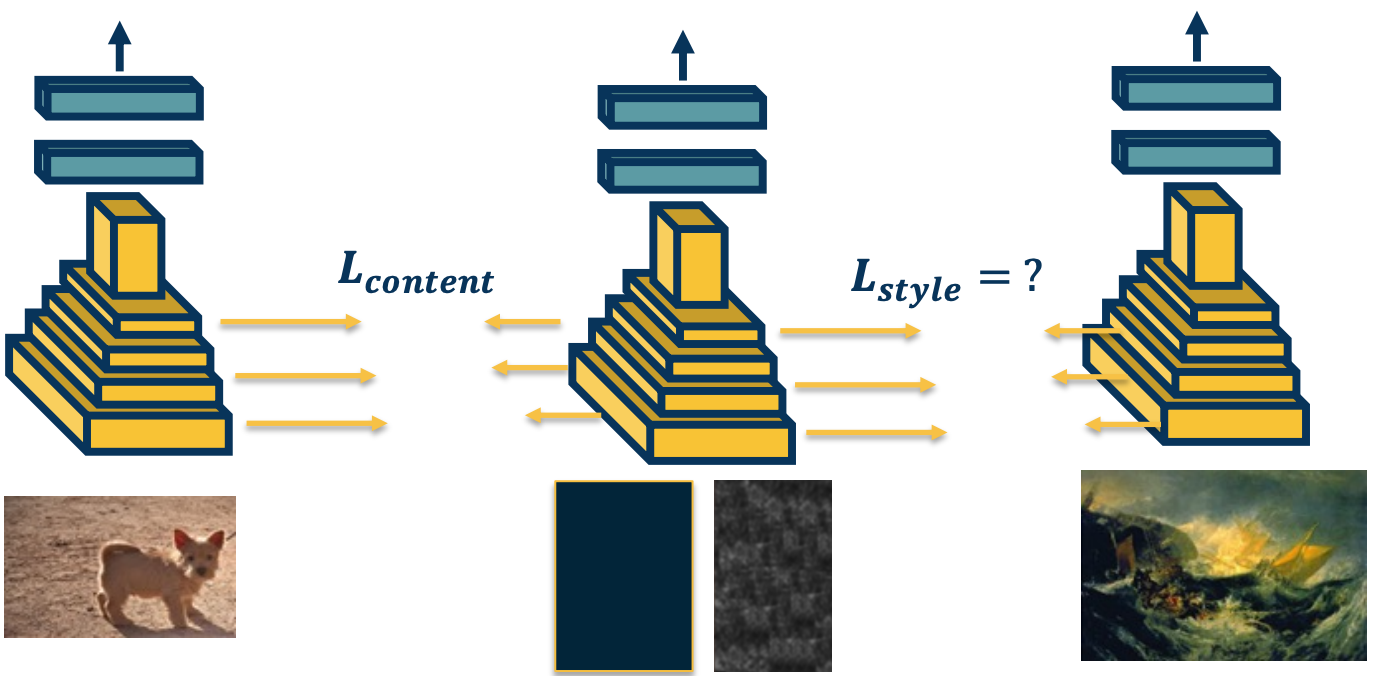
However, it is not clear what this loss function should be - We cannot just use the same loss that we did for the content because it is going to match the content of the second image as well.
Representing Texture
- How do we represent similarity in terms of textures (and not content?).
- There is a long history in image processing looking at these types of problems, specifically around texture generation.
- Key ideas typically revolve around summary statistics.
- For example higher order histograms
- Whatever statistics you use should remove most of the spatial information.
- Because we are interested in not the specific contours or shapes within the image,but just the texture or the style.
- Key ideas typically revolve around summary statistics.
Deep Learning researchers have come up with what is called a Gram matrix and specifically it features correlations across different layers in the neural network. It turns out that these will be sufficiently represent something about texture such that if we match it during our image generation, we can actually generate images with that style.
Gram Matrices
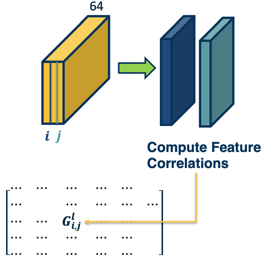
Here how it works - We will take a particular layer in a convolutional neural network and have some set of feature maps. Here, this layer has 64 kernels, so the depth is 64. We will take a pair of channels within this feature map (represented here as i, j) and we will compute the correlation or dot product between the two feature maps.
- Perform an element wise multiplication and then sum it up across the entire channel.
This single value will feed into a larger matrix that represents the correlation between all pairs of channels across this feature map. So the size of this matrix will be 64 by 64.
In mathematical terms:
\[G^l_S(i,j) = \sum_k F^l_S (i,k)F_S^l(j,j)\]Where $i,j$ are particular channels in the output map of layer $l$ and $k$ is the position (convert the map to a vector).
Then, we define a loss function that tries to minimize the difference of the squared difference between the gram matrices themselves. Here we will have a loss with respect to the style where we compute the difference between the gram matrix of the style image with respect to the gram matrix of the generated image.
\[L_{style} = \sum_l (G_S^l - G_P^l)^2\]We will have two losses here, we will have the content loss which tries to match the feature themselves of the content image and the generated image - as well as the style which tries to match the Gram matrix between the style image and the generated image.
\[L_{total} = \alpha L_{content} + \beta L_{style}\]Like all cases when we have multiple losses, we will assign weights between them $\alpha,\beta$. The content loss and the style loss can be across multiple layers in the neural network not just one.
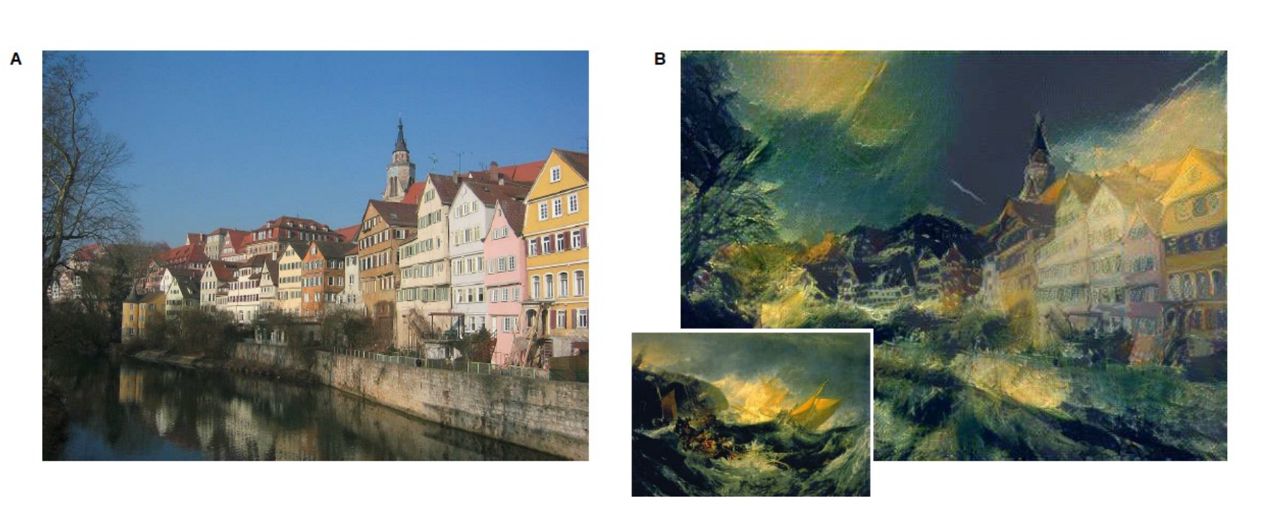
Here is an example of a style transfer - you can see here it is really picking out the details. So the generated image does not have the details of the content but the actual texture or style is matching the particular style image that we have.
In summary,
- Generating images through optimization is a powerful concept!
- Besides fun and art, methods such as stylization also useful for understanding what the network has learned.
- Also useful for other things such as data augmentation
Lesson 8: Scalable Training
Readings
None!
Scaling Deep Learning from Experiment to Production
Pytorch offers some tools such as:
1
2
3
4
5
6

import torch
from torch import autograd

torch.autograd.profiler.profile
torch.utils.bottleneck # Summarize cPython and autograd profilers
torch.autograd.detect_anomaly
- autograd profiler
- shows various performance metric
- Bottle neck
- summarize both the autograd and c python profilers
- Autograd detect anomaly
- returns as soon as a nan is detected during computations
In pytorch there are two modes:
-
Eager mode
- Can type commands which are executed immediately.
- This enables simple debuggable python programs prototyping deep learning code.
-
Script mode
- Programs are converted and ran by a lean just-in-time (JIT) interpreter.
- This is useful for running in Production
- Programs are converted and ran by a lean just-in-time (JIT) interpreter.
Just in time (JIT) can do various types of optimization:
- Algebraic rewriting: Constant folding, common subexpression elimination, dead code elimination, loop unrolling, etc.
- Out-of-order execution: Re-ordering operations to reduce memory pressure and make efficient use of cache locality
- Kernel fusion: Combining several operators into a single kernel to avoid per-op overhead
- Target-dependent code generation: Compiling parts of the program for specific hardware. Integration also ongoing with TVM, Halide, Glow, XLA
- Runtime: No python global interpreter lock. Fork and wait parallelism
Behind the scenes, PyTorch uses different optimized C++ libraries for CPU and GPU. We can extend the library by adding custom C++ operations that can be added in a way similar to pybind11. But using custom C++ operations has the advantage of providing jitability.
Ingest Data
The DataLoader is compatible with two standard python data representations.
- The iterable data set
- Provides each data point one at a time through an iteration process
- support streams or storage when it comes to one data point at a time.
- The map style data set
- Provides a map interface that allows us to access items in any order.
- Because we know the lane, we can also sample randomly because of the flexibility these obstruction provide.
- Because of the flexibility, users often insert preprocessing or data augmentations directly into data set methods.
For more information, refer to the documentation.
Note, you can pin_memory - that is for the data to be stored in the ram.
- Copy from host to GPU is faster from RAM directly. To prevent paging, pin tensor to page-locked RAM.
- Once a tensor is pinned, use asynchronous GPU copies with to(device, non_blocking=True) to overlap data transfers with computation.
- Script mode: TorchScript A single Python process can saturate multiple GPUs, even with the global interpreter lock.
Use Multiple GPUs and Machines
There are two different types of parallel
- Data parallel
- data is distributed across devices
- Model parallel
- model is distributed across devices
Look up the necessary documentation depending on which type of parallelism you require.
Distributed Model Parallel
The case for completely distributed model parallel requires more flexibility - we want to share the model across GPUs living on different machines.
RPC is remote procedure call and on top of it lives the reference counting protocol, remote objects to access, distributed autograd and distributed optimizers.
Again, look up the required documentation if you need to do so (unlikely in this course) based on each of the following scenarios:
- Single-device training: if the data and model can fit in one GPU, and training speed is not a concern
- Single-machine multi-GPU DataParallel: if there are multiple GPUs on server, and want to speed up training with minimum code change
- Single-machine multi-GPU Distributed Data Parallel: for further speed up in training if willing to write a little more code
- Multi-Machine Distributed Data Parallel: to scale across machine boundaries
- TorchElastic: if errors are expected or resources can join and leave dynamically
Lesson 9: Advanced Computer Vision Architectures
Readings
Image Segmentation Networks
We will start moving beyond image classification where we take an image and output a probability distribution over the classes or categories. We will start talking about other computer vision tasks such as image segmentation or object detection.
Computer Vision Tasks
Other tasks we may want to perform is semantic segmentation - we want the same probability distribution but for each particular pixel. Note that we are not distinguishing instances here (does not care whether the pixel belongs to same or different cars, we only care the pixel belongs to a car).
We might want to do instant segmentation where we actually have a unique ID for each instance as well.
Another task is object detection. We are not looking at individual pixels, but rather looking at bounding boxes. That is for each object in the scene, we want a bounding box around that object and a probability distribution over the categories.
These are not always independent, sometimes network can combine to estimate all or some subset of them.
Segmentation tasks
Given an image, we really want output another image.
- Each output contains the same width and height, but a class distribution per pixel.
- This is more generally referred to as an image to image problem.
- We have an input tensor with width and a height and a number of channels (typically 3 for regular RGB) and we want the output to essentially be another tensor with the same width and height because we are trying to classify each pixel and the depth is the number of categories.
Here is a depiction of it looks like:
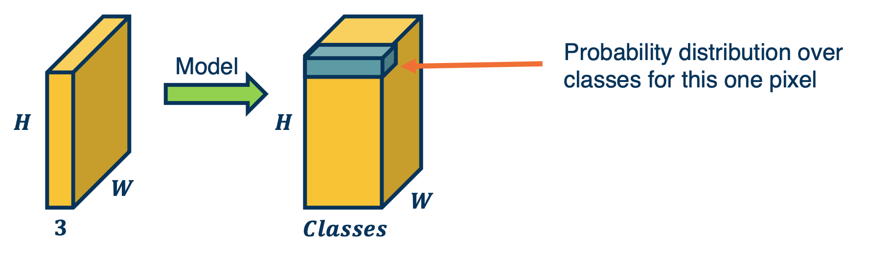
This is drastically different from what we have done before - thus far we have applied a CNN to an image and this creates downsampled feature maps at the end of the convolution layers and are then fed into fully connected layers.
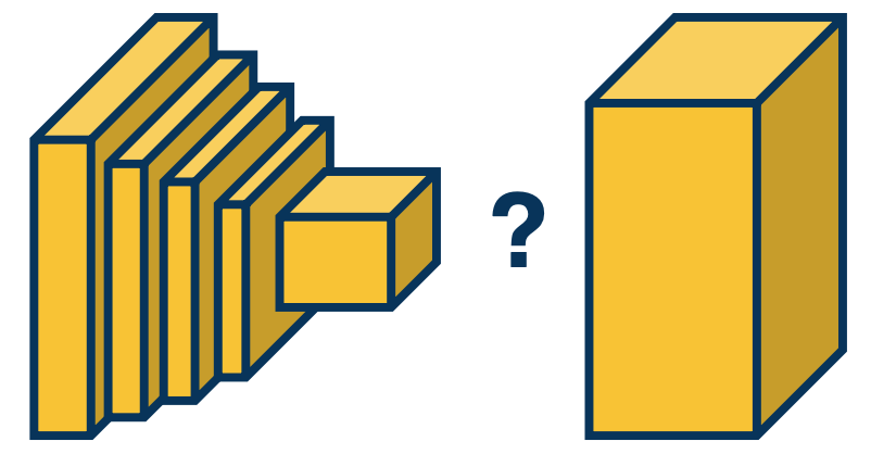
The CNN performs some dimensionality reduction both through convolution operations and also through pooling operation. The question is, how can we perform up sampling here?
- We want to still extract meaningful, abstract high level features.
- However, we want then convert those features into some estimates for these tensors.
Idea 1: Fully-Convolutional Network
One reason fully connected layers are not applicable to segmentation problems is that they throw away explicitly spatial information. The output of FC layers is in the form of vectors! They are no longer spatially organized, similar to how the images were.
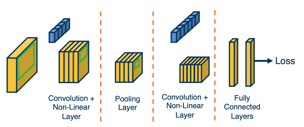
The neural network can still retain some spatial information, for example by learning weights that are specific to different regions of the output feature maps at the last convolution layer. But it certainly not an explicitly spatial representation.
Thus, one idea is just to get rid of fully connected layers all together - perhaps we can devise a fully convolutional neural network that does not have fully connected layers and maybe still output something resembling segmentation outputs.
Converting FC Layers to Conv Layers
It turns out you can convert fully connected layers into a convolution operation. This is because convolution operations are very similar linear operations to fully connected layers as we have discussed before.
What we can do is just take the fully connected output nodes and reshape them back into the same sizes. This can be seen as a convolution operation because we can just have the kernel be the same exact size of the input.
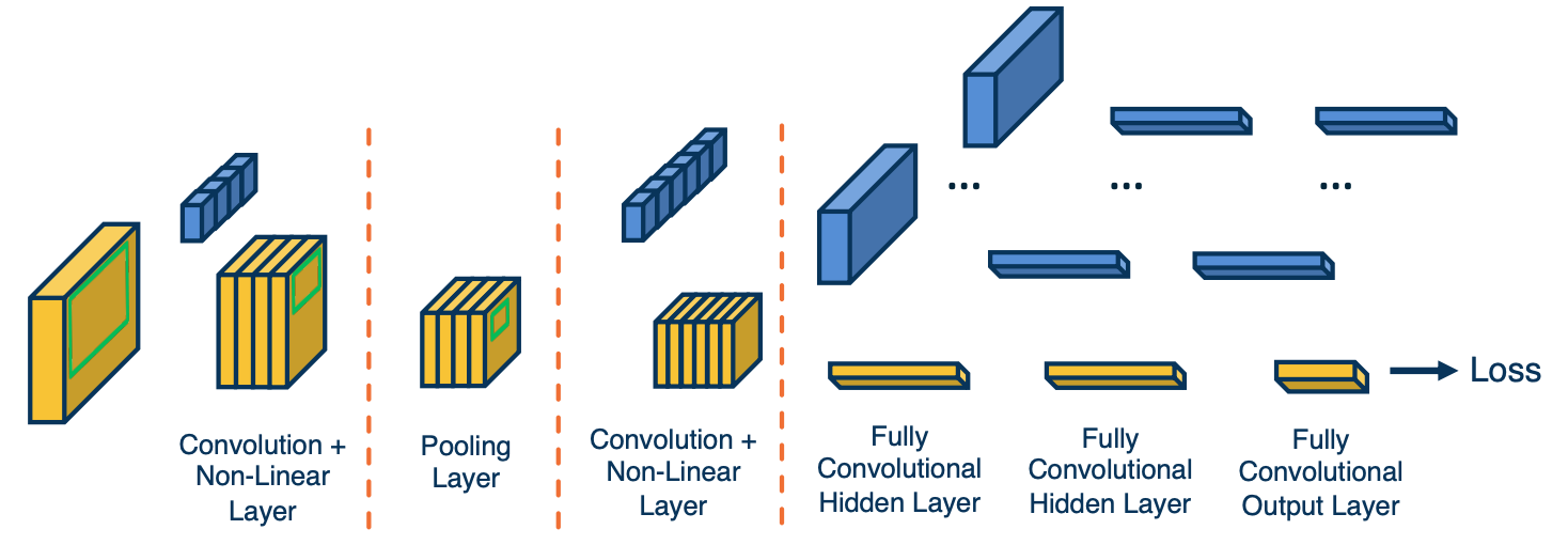
If you see here there are some sets of output feature maps at the end of the last convolution layer. And then we will have kernels which are shown in blue with the same exact size as that input to the next layer. So rather than have a fully connected layer, we will have a fully connected convolutional hidden layer where each kernel is essentially representing each output node.
This can be thought of just taking that kernel just dot product it was the entire input, and for that we get one scalar output. This is exactly equivalent to $Wx+b$ in the fully connected layer that we talked about. We can also do this for other layers as well.
Same Kernel, Larger Input
Mathematically, the representation of a fully connected layer or a convolution layer where the kernel is the same size as the input are equivalent.
Why would we want to do this trick?
It turns out that this allows us to be no longer dependent on a particular input size and we will show how this is useful for segmentation.
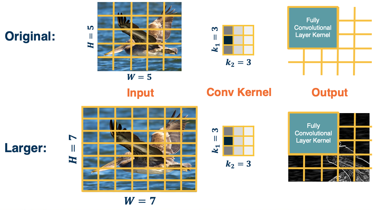
For example, suppose that we have an original input size here 5 by 5 image, and we have a kernel that we have learned a 3 by 3 image - and this results in an output size of 3 by 3. When we have a fully connected layer after this, or after we have converted it to a fully convolutional layer. We will have a kernel that is exactly the size of this output. So we will have a fully convolutional layer kernel that dot producted with that to produce one output node in the fully connected or fully convolutional layer. We can have multiple of these if we want multiple output nodes.
It turns out that if we feed it a larger input, as we know it, since it is normal convolution, the output map at the last convolutional layer will be bigger. This is because the convolution operation is defined by the striding operation and has nothing to do with a particular input size. So if we retain the same fully convolutional layer as before, we will now have a smaller classifier with respect to the new larger output sides. You could see that now we will have a larger output - a 3 by 3 from this fully convolutional layer kernel being strided across this new larger input.
Inputting Larger Images
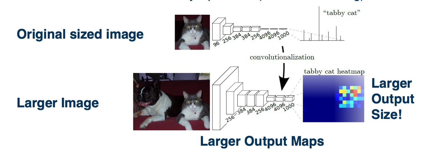
This matters because we actually just see this as striding a classifier across the larger outputs. We can actually use this to get a segmentation output. Specifically, we can take a smaller sized, lets say the normal image net classifier sizes which are typically 224 by 224, shown here where it says original size image and we just learn a normal CNN. It can have normal fully connected layers.
We now feed it a larger image and we convert the fully connected layers to fully convolutional layers. We will just reshape those weights to be the size of the inputs. When we run this larger image through the CNN, we will get a larger output at the last convolutional layer and we will stride this original classifier that we learned and we will get multiple outputs. This corresponds to applying the classifier at different positions in the image. This is a very segmentation like output, that is for each position in the image, we get an output of what the class label is. Of course, the size of this heat map that is shown here on the right is going to be dependent on how much you are enlarging the input image size.
If you only enlarge the input image size by a little bit,you will get a very tiny heat map. If we use much larger images, then we will get much larger heat maps -> Then we will essentially get a segmentation output, where each pixel in the image we can get what class or category in that image.
Notice that we do not quite get every pixel here, since it is still down sampled, the output is still going to be smaller than the actual image. You could do various tricks such as upsample, apply normal image processing methods to take this heat map and resize it to the larger image size and achieve some probability distribution across the original image.
Idea 2: “De”Convolution and UnPooling
Now, the fully convolutional neural network that we devised for segmentation is perhaps still not ideal. Even though it gets us some coarse segmentation output that we can then up sample, it is still not going to be that high resolution and we also have to feed in much larger images to get that output.
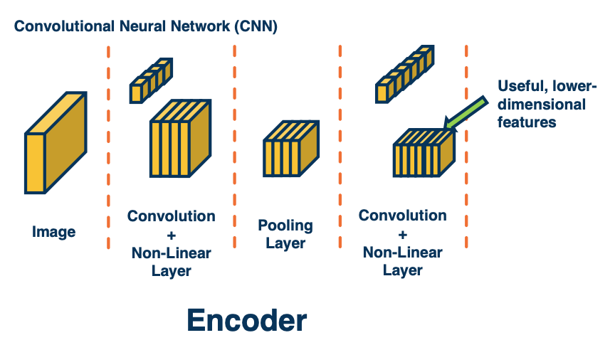 We can develop learnable or non-learnable up sampling layers!
Instead, we could try a different idea. Here, we might think about how we can devise layers that actually perform up sampling rather than down sample? Traditionally when we looked at the convolution and max pooling layer, these resulted in smaller images at the output. We continue to apply this and got small feature maps by the end. This is called an encoder - we are encoding the image into highly relevant abstract features that are important for whatever task we want.
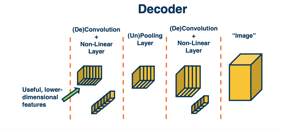
So, we could try to think about how to develop what is called a decoder. That is, we want to take in those small feature maps, which represents very important features and try to use them to up sample - to generate more and more high resolution outputs that eventually are the size of the original input image. This is called an encoder-decoder architecture. We will see these both in computer vision as well as natural language processing and other applications.
Now, how can we actually do this? It turns out we can actually do some sorts of inverses of the traditional layers that we had.
- transpose convolution or loosely termed deconvolution
- unpooling layer
- does something slightly similar but results in a larger output rather than a smaller output.
Max Unpooling
Remember this is max pooling:
\[X = \begin{bmatrix} 120 & 150 & 120 \\ 100 & 50 & 110 \\ 25 & 25 & 10 \\ \end{bmatrix} \xrightarrow{\text{2x2 max pool}} Y = \begin{bmatrix} 150 & 150 \\ 100 & 110 \end{bmatrix}\]The idea in unpooling, we copy the value to position chosen as max in encoder, fill reset of this window with zeros. For example:
- $y(0,0)$ is from $x(0,1)$
- $y(0,1)$ is from $x(0,1)$
- $y(1,0)$ is from $x(1,0)$
- $y(1,1)$ is from $x(1,2)$
At the decoder step:
\[X = \begin{bmatrix} 300 & 450 \\ 100 & 250 \\ \end{bmatrix} \xrightarrow{\text{2x2 max unpool}} Y = \begin{bmatrix} 0 & 300+450 & 0 \\ 100 & 0 & 250 \\ 0 & 0 & 0 \\ \end{bmatrix}\]Notes:
- For windows that overlap that have the sam max indices in the same spot, we will just sum them up.
Symmetry in Encoder/Decoder
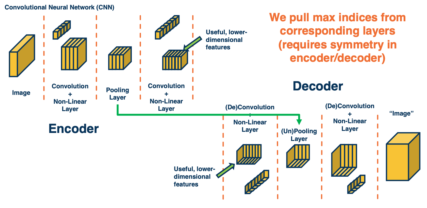
You might wonder - What does it mean to have a pooling and unpooling layer correspond? What we are going to do is we are going to have an encoder, which may consist of multiple convolution and pooling layers and then have a decoder that are symmetric to the encoder. In other words, the architecture of the decoder will be completely the reverse of the architecture of the encoder.
The result is essentially an architecture that allows us to do unpooling across the layers by remembering the locations of the corresponding Boolean.
“De”Convolution (Transposed Convolution)
One issue with max unpooling layer is there are no learnable parameters. So we are not really learning how to upsample. All we are doing is taking the max indicies in the encoder stage and applying them at the decoder stage to upsample images. The next question is, can we actually apply a similar operation as a convolution where you have a learnable kernel and perform upsampling?
Transposed Convolution (also known as “deconvolution”, fractionally strided conv) - Take each input pixel, multiply by learnable kernel and “stamp” it on output.
(Note, deconvolution is not a great name because it means something very specific mathematically that is different from what we are doing here)
Transposed Convolution Example
Given the following:
\[X = \begin{bmatrix} 120 & 150 & 120 \\ 100 & 50 & 110 \\ 25 & 25 & 10 \\ \end{bmatrix} K = \begin{bmatrix} 1 & -1 \\ 2 & -2 \end{bmatrix}\]After we incorporate $X(0,0)$ - i.e we take the $X(0,0) \cdot K$ and “stamp” it on the output.
\[\begin{bmatrix} 120 & - 120 & 0 & 0 \\ 240 & -240 & 0 & 0 \\ 0 & 0 & 0 & 0 \\ 0 & 0 & 0 & 0 \\ \end{bmatrix}\]and we incorporate $X(0,1)$, take $X(0,1) \cdot K$ and also stamp it:
\[\begin{bmatrix} 120 & - 120+150 & -150 & 0 \\ 240 & -240 + 300 & -300 & 0 \\ 0 & 0 & 0 & 0 \\ 0 & 0 & 0 & 0 \\ \end{bmatrix}\]and so on. Again, contributions from multiple windows are also summed.
Symmetry in Encoder/Decoder Part 2
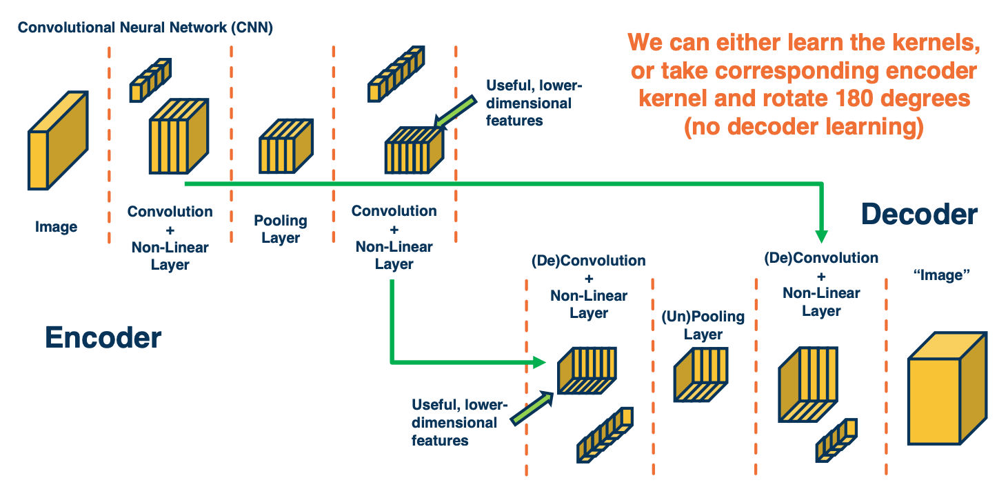
Because we have a symmetric encoder and decoder, we can actually do two variants of this.
- The first is to have the kernel learned and the kernel values will be learnable parameters and we can backpropagate through them.
- The other alternative is actually to not learn the kernels at the deconvolution or decoder stage. What we can do is take for each deconvolution layer, take the corresponding mirrored convolution layer in the encoder and then take that kernel that was learned or those kernels that were learned and flip them 180 degrees and then apply them in the decoder.
These two variants exists but typically the kernels are learned.
Transfer Learning
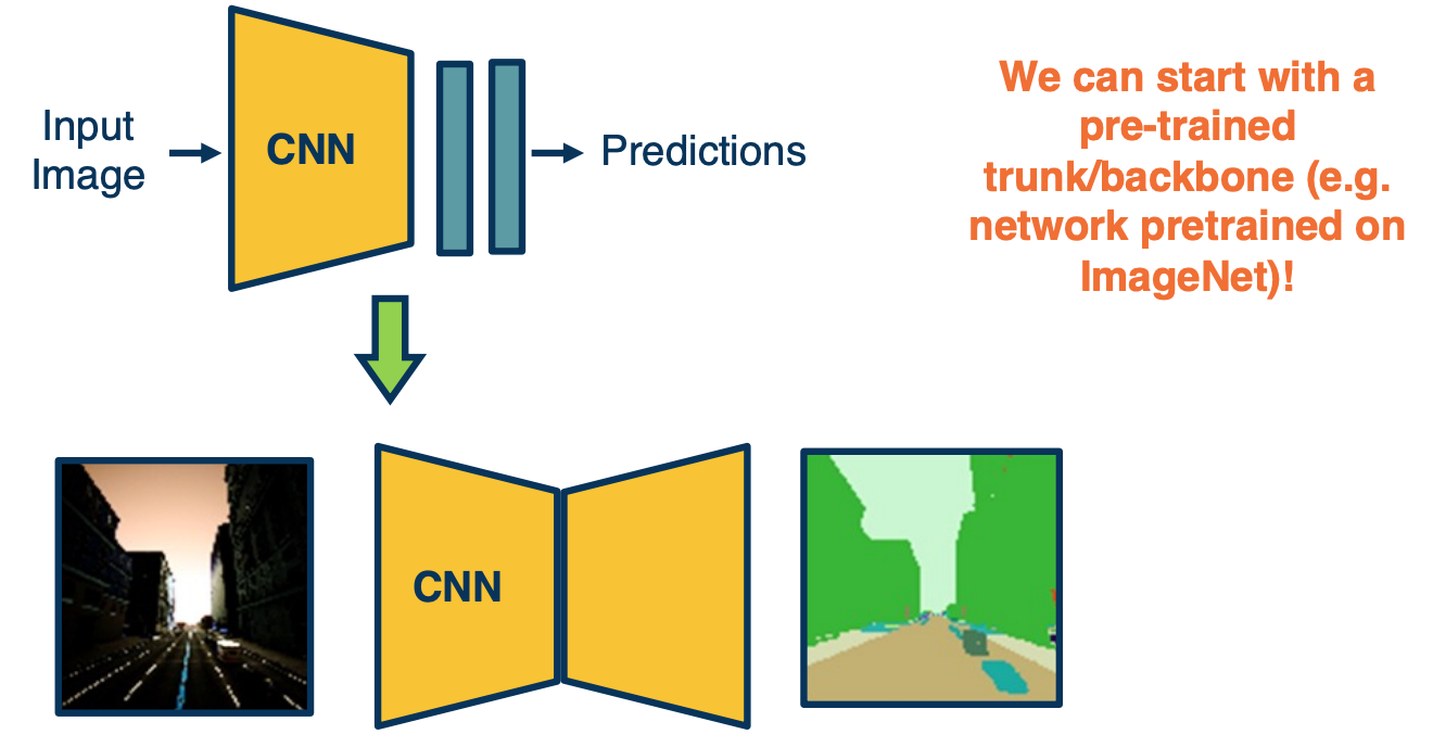
Because we are using a normal convolution neural network for the encoder, we can actually use transfer learning here again. We can train a convolutional neural network for image classification, let’s say on a large dataset such as image net (which has 1 million examples over 1000 object categories), and optimize those weights for the image classification loss. We can then take those learned weights and copy them to the encoder and we can mirror the architecture for the decoder and initialize those randomly.
Then we can jointly optimize the encoder and decoder given ground truth if we have it, for a segmentation task. Note that we will also use cross entropy, except that we have a probability distribution over the categories for each pixel. So we will have that many losses that all get into the optimization during backpropagation.
U-net
You can also use alot of the ideas that we had for image classification. For example, residual neural networks use the idea of skip connections. We can also do this for encoder-decoder networks. This is what is called a U-net.
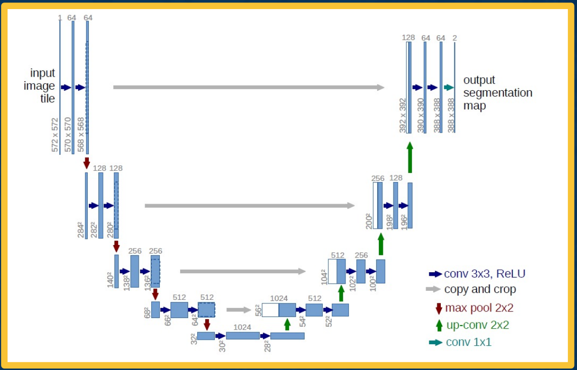
It is the same thing as what we had before, we have an encoder part and then some bottleneck features and then we have a decoder part. Except here we are not using only the bottleneck features. We can have skip connections where you take the feature maps from various parts of the encoder and actually concatenate them with various parts of the decoder. What you are doing here is combining information both from the encoder at multiple scales that is at multiple resolutions of information because the feature maps get smaller and smaller and you are combining that with the upsampling that we do for the decoder. This is a very successful architecture for various types of segmentation tasks.
In summary,
- Various ways to get image-like outputs, for example to predict segmentations of input images
- Fully convolutional layers essentially apply the striding idea to the output classifiers, supporting arbitrary input sizes
- (without output size requiring particular input size)
- We can have various upsampling layers that actually increase the size
- Encoder/decoder architectures are popular ways to leverage these to perform general image-to-image tasks
Single-Stage Object Detection
We will talk about Object detection and specifically single stage methods, that take images try to directly output a set of bounding boxes with predictions for each of them.
Object Detection Tasks
Given an image and we want to output a list of bounding boxes with probability distribution over classes per box.
There are several problems here:
- Variable number of boxes
- Do not know how many objects will appear in these images.
- Need to determine candidate regions first
- Where are they in positions and scales of the different possible object location in the image
We can make architectural changes in order to make this happen. For example, we can use the same idea of fully-convolutional neural networks
- Use imageNet pre-trained models as backbone (e.g taking in 224 x 224 image)
- And then we can feed in a larger image and classifications for different windows in the image.
But we are only getting the probability distribution over the classes at the end! We are not looking for a probability distribution over the classes for each pixel. What we want is actually an estimate of the bounding box. (A bounding box is where the upper left corner of this object starts and the width and height of the object which is one representation for a bounding box). You can have four numbers representing this bounding box, x,y,h,w.
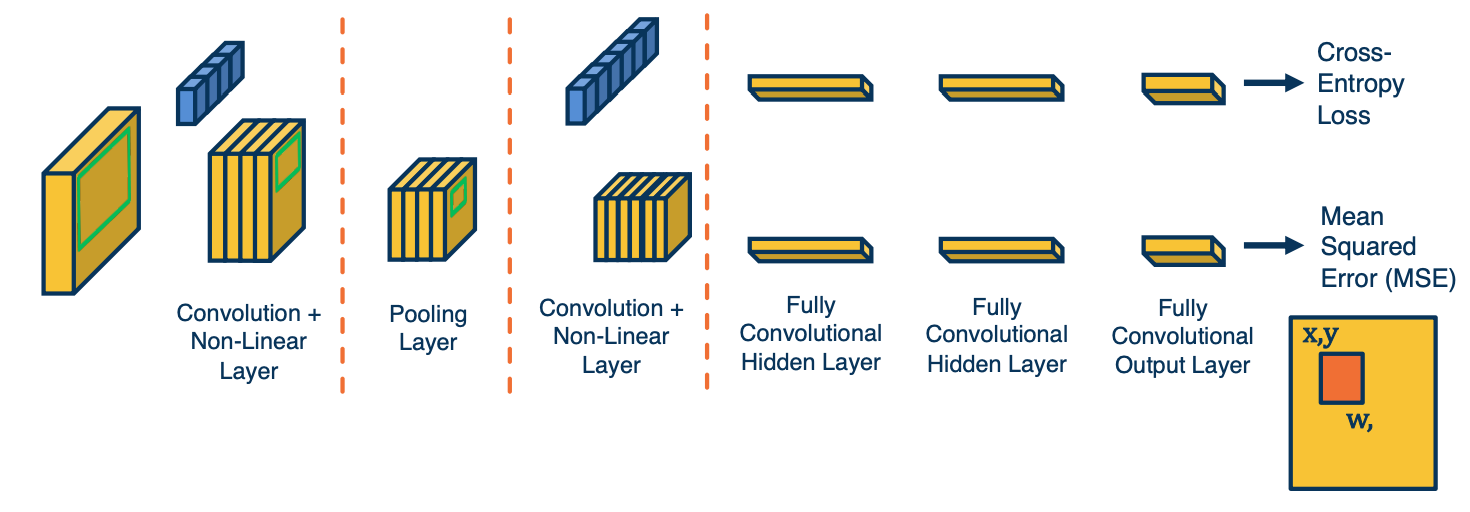
What we can do is to have a multi-headed architecture.
- One part predicting distribution over class labels (classification)
- One part predicting a bounding box for each image region (regression)
- Refinement to fit the object better (outputs 4 numbers)
- Both heads share features! Jointly optimized (summing gradients)
- We can tie these things in the same joint computation graph and optimize for both the classification task and regression task for bounding boxes.
- This will imply that we have two loss function.
- For regression we can use MSE.
- We can then use a weights to average the two loss function.
This is what it will look like:
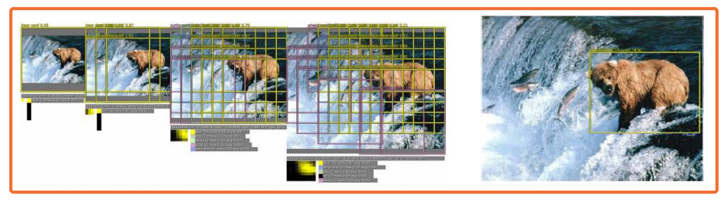
We will actually feed in multiple images of the same thing, but at different scales. That is will take the same image and either downsample or upsample it, using traditional image processing methods. We will feed all of these into the fully convolutional neural network. For each of those, it will give us across some gridded pattern, a set of predictions for each grid element, which has classification probability distribution, as well as regression to a bounding box that is x,y, width and height.
What you will notice here is first of all it is gritted because of the fact that we are using a fully convolutional neural network and it results in small feature maps at the last convolution layer, and we are essentially striding a classifier or regressor across that small feature map. Thus, by definition, it will essentially lead to grids in the input image, when we figure out what receptive field each of those convolution feature maps have. Another thing oyu will notice is that this may again low resolution similar to before, the output is really going to be a set of heat maps. This may be too low resolution for things like object detection.
There is going to be a bunch of tricks in this paper that you can look at that actually tries to make this higher resolution outputs (decrease subsampling ratio). Another thing to mention is that you will have lots of different bounding boxes and many of them may have low probabilities for different objects, so you might be able to filter them out. But in the end you will have multiple bounding boxes, especially around actual object.
In computer vision, there is a whole set of techniques that take a lot of different predictions in similar locations all with probabilities associated with them, and combines it into one or few actual boxes. This is called Non-Maximal Suppression (NMS).
Single-Shot Detector (SSD)
Over the years, a number of refinements have been made over these architectures. For example the single shot detector or SSD. SSD use a similar idea of grids as anchors, with different scales and aspect ratios around them.
SSD will impose a grid over the input image, and this corresponds to some grid over the convolutional feature maps at that last convolution layer. And then for each position in that grid will actually estimate some set of bounding boxes of particular shapes or aspect ratios. (This is a pure hyperparameter).
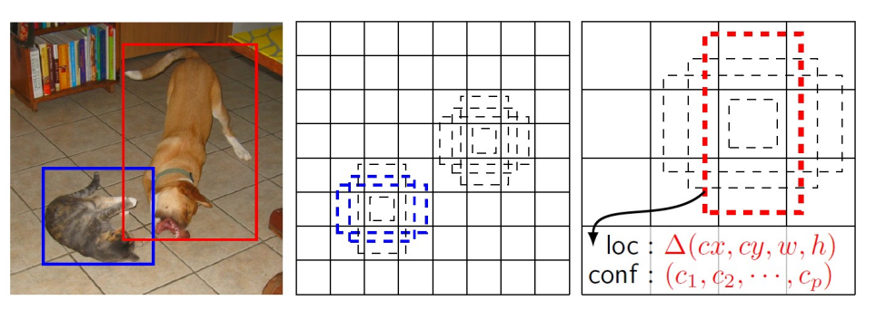
In the image above, there is four different bounding boxes here as dotted lines that we estimate. Then, for each of those bounding boxes, we estimate refine bounding box (x,y,width,height) as an output of a neural network as well as a confidence that is probability distribution over classes. Because we have a fixed number of these, because the grid is a fixed number of elements, and each grid location has a fixed number of bounding boxes around which we estimate this. You can actually just have one big neural network that outputs this directly:
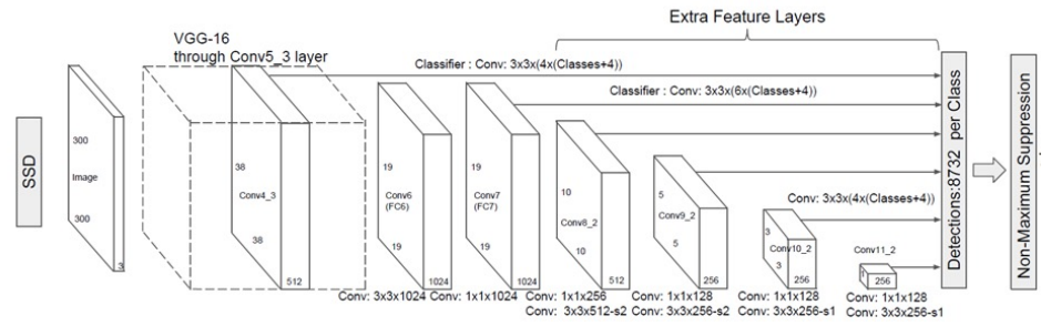
So there is various tricks that you can use to increase the resolution of this, such as skip connection or multi resolution idea as well. Here you will notice you actually estimate these across a number of bounding boxes in different layers. You do not actually impose this grid on one particular feature maps but actually impose this on multiple feature maps across the depth of the network. So closer to the input you will have higher resolution one since the larger size outputs allow you to do that. Whereas deeper inside the network, your convolutional neural output maps are much smaller, and so your predictions are going to be smaller as well. You then combine all of the predictions that the neural network makes across all of the different layers and then you perform non maximal suppression. In this case if you notice you will have 8732, a fixed number of prediction and you can apply NMS to that to produce a small number of bounding boxes, for example around the cat and the dog.
YOLO
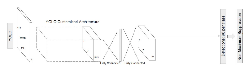
There are also other architectures such as YOLO (you only look once) that has a similar idea. You have an input image and you want to essentially make predictions for each grid location across those images or across the feature maps. In this case, the only difference is that we are going to use some customized architecture. SSD actually uses a convolutional neural network backbone that is pre trained on ImageNet such as resnet, but in yolo there is a custom architecture that eventually leads to a fully connected layer, making predictions for a fixed number of grid locations.
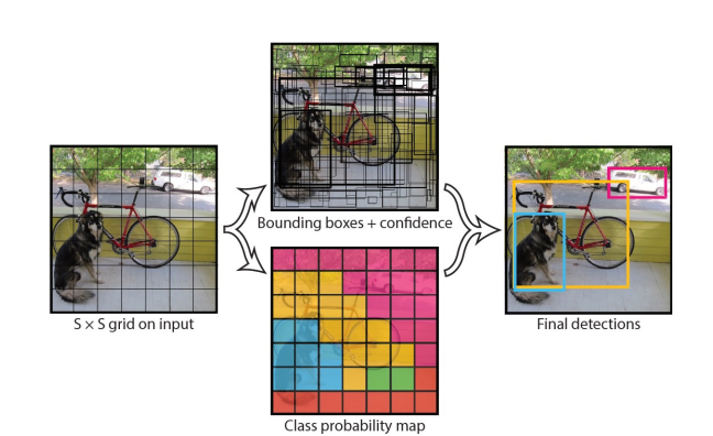
There are various trade offs between accuracy and computation across all of these architectures.
Datasets
The way we evaluate these through large data sets. There is a dataset called COCO which has a lot more objects per image. Imagenet typically just has one while COCO have somewhere between 3 to 7 objects per image. There are alot more data and categories in COCO, 80 compared to prior object detection datasets such as Pascal VOC.
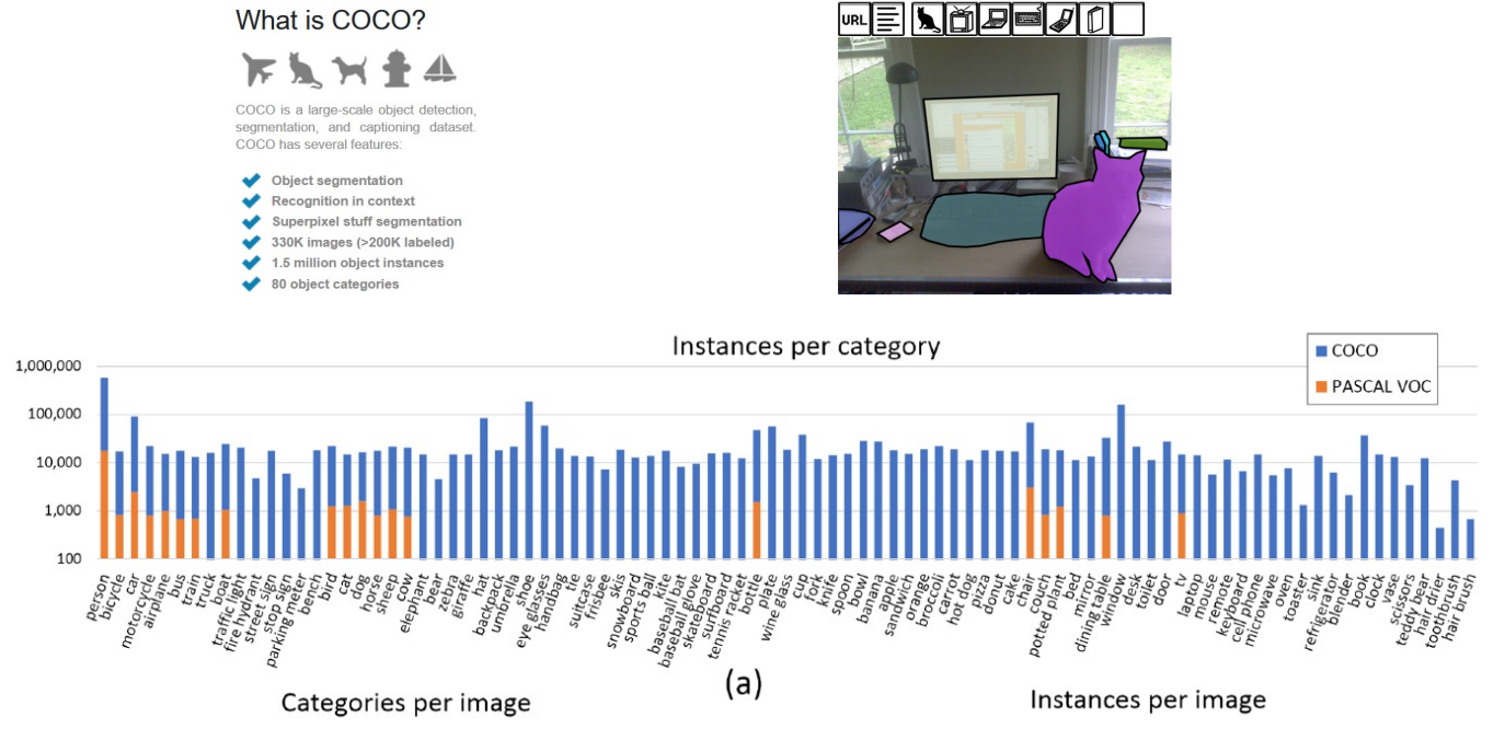
Here you can see a distribution or histogram across all of these different categories.
Evaluation – Mean Average Precision (mAP)
There is also various ways to perform evaluation. In the case of bounding boxes the metrics are much more complicated.
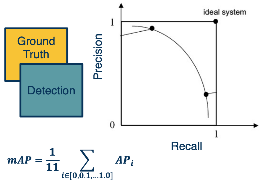
Here is one example:
- For each bounding box, calculate intersection over union (IoU)
- Keep only those with IoU > threshold (e.g. 0.5)
- Calculate precision/recall curve across classification probability threshold
- Calculate average precision (AP) over recall of [0, 0.1, 0.2,…, 1.0]
- e.g at each recall point, calculate the precision and store them in an array and average input.
- Average over all categories to get mean Average Precision (mAP)
- Higher is better
Over many years, many different architectures have been developed - there is lots of trade offs that you can make. Typically these represent on the x-axis some form of computation complexity either flops floating operation per second (FLOPS) or frames per second (FPS). On the Y-axis you could show the mean average precision.
There is various types of architectures such as the YOLOs which have pretty good trade offs. There is a new variant called PP-YOLO which came out in 2020 that also has a pretty good trade off, you can go up to 130 frames per second on a good GPU. There is also new architectures based on efficient net.
Two-Stage Object Detectors
- One stage that gives us the region of interest
- parts of the image that might contain the object
- Another stage that performs classification and regression to better bound box.
R-CNN
Instead of making dense predictions across an image, we can decompose the problem into two steps:
- Find regions of interest (ROIs) with object like things
- Regions that have a high probability of having some sort of object in them, as opposed to being part of the background.
- Classify those regions (and refine their bounding boxes)
- Specifically we can take each region of interest (corp in the image) and we can resize it to take whatever size that is input to the CNN (for example a pre trained image net model). Then, we can obtain predictions. We can do this for a batch of data and then backpropagate to optimize the model.
Extracting Region Proposal
Now, there is a question of how we find these regions of interest. In some sense, this is the biggest problem that we have for object detection. It turns out we can actually use unsupervised (non learned!) algorithms to find these candidates.
These were developed before the resurgence of deep learning. Specifically we can perform things like unsupervised segmentation of dimensions.
- Group pixels together in order to find symmetrically coherent pieces of information in the image that may correspond to objects. Or, they may be things like patches of grasses and so on.
- We can do this at multiple scales - take the same image, resize it to be bigger or smaller, and then extract these segmentations and then we will combine all that information to get a set of candidate bounding boxes, which may be around some objects.
For example this algorithm shown here is called selective search.
There are several downsides to this algorithm.
- First, it is really slow - it takes one or more seconds per image to extract these bounding boxes.
- Second, they return thousands of boxes, mostly of background or at least parts of objects and not the whole object itself.
Now they do return scores typically but the scores are not very good. In other words, in order to get most of the objects, you have to have a pretty low threshold and you will still end up getting at least hundreds or thousands of boxes.
Another problem with this overall approach is finding candidates and then feeding each candidate through a CNN is going to be really slow. If we feed hundreds of images or crops within an image to a CNN, then it is going to take a long time for just one image to process.
Inefficiency of R-CNN
 Computation for convolutions re-done for each image patch, even if overlapping!
If you think about it, the biggest problem here is that we are wasting a lot of computational resources actually computing the exact same thing, because we are taking a bunch of different corps within an image and a lot of these crops are actually overlapping. Clearly, across thousands of boxes, you will have lots of overlap. If you think about the way convolution layers work as you are striding a kernel across these images, you are actually redoing the computation. For example, for the parts that are overlapping, you are computing the dot product with the kernel for the same piece of image with the same kernel.
Fast R-CNN
What we can do instead, is take the image and feed it through parts of a CNN - that is up until the last convolution layer before the fully connected layers. We will only compute this once and the output of this will be a set of feature maps. Then, given a crop or region in an image, we will find the mapping between the pixels in the image and exactly what pixels in the feature maps they affect. (Think of this as pre computing everything once, and then find the mapping instead of redoing the computation)
Remember, we can compute this, we know given a feature map pixel, what is its receptive field? That is the set of pixels in the input image that is affected by it. And so we can just do this, we take the corp, compute the specific region within the feature maps that crop corresponds to, pull out essentially those stands of features, and then feed that into the fully connected layer. In doing this we are really doing the computation and feature extraction only once. There is one problem with this though; if you have different regions of interest in the image that have different sizes, they will correspond to different sizes in the feature maps. And so since fully connected layers require a fixed input size, this is an issue.
ROI Pooling
To overcome this, we can do something that is called ROI pooling, and this is part of an algorithm that is called Fast R-CNN. It is similar to R-CNN, where we are taking regions of interest and feeding them through a CNN but it is again, doing the same trick (which is computing the convolutional layers only once).
What we are going to do is take whatever sets of feature maps and only take the parts that corresponds to the particular corp in the input space and we are going to grid it. So we are going to have a fixed number of grid elements. In this case a four by three, so 12 grid elements. And for each of these grids elements, we will take a max operation.
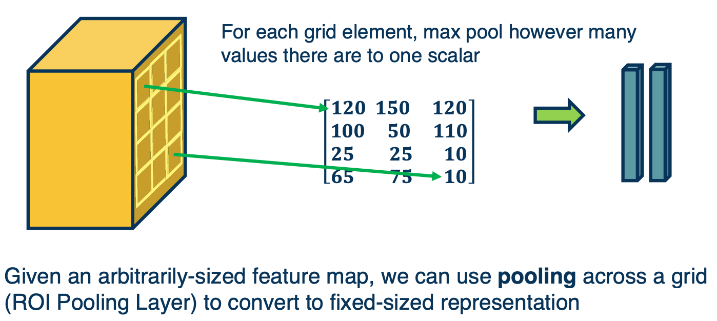
Here we see the upper leftmost grid element, may have multiple values in that little yellow box, but we will take the max and maybe that is 120. Similarly, we wll do this for all location. If you notice that does does, is it actually equalizes the input size. That is because we are fitting a fixed size grid onto the feature maps, the output will be fixed size, and now we can feed them into a fully connected layer. Notice that you can back propagate through this, similar to any max pooling type layer.
Fast R-CNN part 2
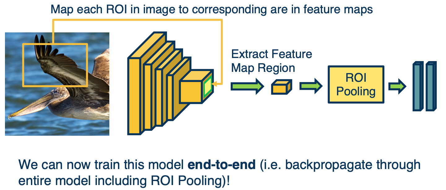
So now we can train this model end to end using backpropagation. That is we have an image, we compute the convolution parts of the CNN, we extract some feature maps that result from that and then we have a set of bounding boxes or ROIs that come from whatever other algorithm that is not learning based. We then extract those feature stands that correspond to that, and then feed those to ROI pooling and fully connected layers. Again, because we can back propagate through the ROI pooling as well as all parts of this process, we can actually just optimize the entire thing. We can back propagate all the way to the features and optimize them as well.
Faster R-CNN
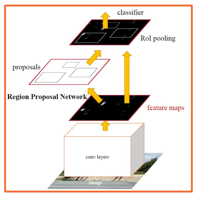
There is a follow on algorithm called faster R-CNN. The idea here is to make use of deep learning to do everything.
- Rather than have a separate non-learning based algorithm that gives us these regions of interest,
- We will instead use a region proposal network or RPN.
- This RPN will take the same features that the convolution parts of the CNN extract, and will estimate a set of bounding boxes along with what is called an objectness score.
-
objectness score is the probability that there is some interesting object in there.
- And potentially a refined bounding box.
- Have the RPN regress from the features to a set of bounding boxes and then select the top K of them with the highest probability of having some object in them and continue with the process.
- Perform ROI pooling on the same features, and then perform classification and regression again.
- We now have 4 losses:
- Classification object miss score for the region proposal network,
- bounding box regression loss,
- Classifier loss that classifies not between object or not object but across however many categories we have
- Lastly, another bounding box regression or refinement.
- Note some parts (gradient w.r.t. bounding box coordinates) not differentiable so some complexity in implementation.
- For example, it is not clear how to find the gradient of the loss with respect to the bounding box coordinates.
- For example if you think about moving the bounding box a little bit, because you are changing the weights that map the features into the bounding box that is the regression network, it is not clear how your loss changes. Because you are actually changing the bounding box itself, which means you are taking different inputs, different pixels, and then those get fed into ROI pooling and you are performing classification.
- One way to do this is just alternate the training, that is trained to RPN and then train the classifier and then alternate these two steps.
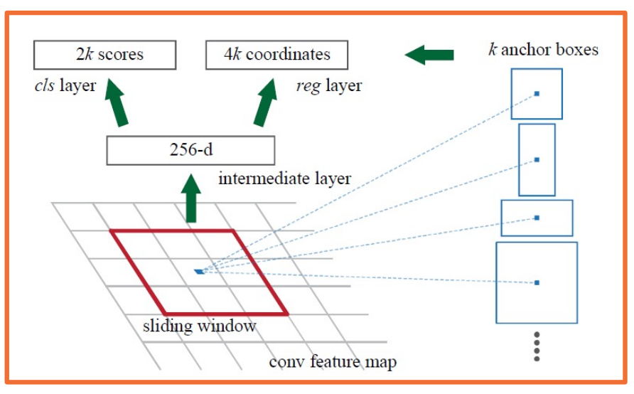
Now we still have the problem that the region proposal network cannot really have a function that regresses from the feature maps to an arbitrary number of boxes. And so here, we will use the same trick that we used for YOLO and SSD, that is we will have a grid on the feature map, which is actually a grid also on the input because of the receptive field and calculations. What we will have our anchor points, which are centers of these grids, and for each anchor will have k anchor boxes stemming from them. These are boxes of various size and shapes, whose centers are in this anchor center. And again, the size, the shape, and number of anchor boxes that you have are all hyper parameters.
And so here, we will learn a function that directly regresses from the feature maps to a 256 dimensional hidden vector (in this case), and then regresses to 2k scores. It is 2k because we are classifying between two classes, object like or not object like, this is called the objectness score. We will also regress to 4k coordinates, again it is because of four coordinates per bounding box where we are refining the object bounding box. Because these anchor boxes might actually not perfectly overlap on top of the objects that we care about. And so again, this allows us to explore boxes of various sizes and scales along with objectness scores and refined bounding boxes. And doing this in a way where we are not outputting a variable number, but rather a large number. And then we can take the top objectness scores, the bounding boxes out of all these that have top objectness scores, and take the top end of them. That is we will filter out the rest that have low object scores.
These will be the regions of interest that are fed to the other branch, which is the classification branch.
Mask R-CNN
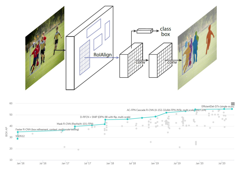
There are other advances that have been made since - there is a large number of different architectural changes that you can make. You can also combine it with various other types of computer vision tasks.
For example, Mask R-CNN performs the same thing as faster R-CNN, except it also ahs a mask that it learns, that is a segmentation. So for each region of interest, it not only tells you what is the object that is in that bounding box, but it also tells oyu exactly which pixels wi thin that bounding box actually touches the object, because there may be some background pixels (like grass and so on)
Over the years, there has been many algorithms that have improved the mean average precision of object detection and segmentation in data sets such as COCO. On the lower right, you could see a nice graph. This is from a website called papers with code, which tracks the state of the art across various deep learning, another AI machine learning tasks. Here you could see it progressively increasing where a Mask R-CNN is actually not that high, you can get approximately 40-45% MAP, and then efficient Det which is a new architecture based on efficient net, which is a classification architecture that can get much better.
Again, there is a large space here between computation and accuracy as well.
In summary,
- Two stage object detection methods decompose the problem into finding object-like regions, then classifying them.
- At both steps, bounding boxes are refined through regression
- And so for Faster R-CNN and other variants where the region proposal network is also learn, we will have at least four losses, classification loss for objectness, bounding box regression at the region proposal network.
- These candidates that are highly scored will then be fed through the classification part, which will output classification across the categories and then another regression to further refine the bounding box.
- If you notice, we can keep adding various losses such as Mask R-CNN has additional losses for the foreground background mask.
- These algorithm also have alot of hyperparameters. You will see 30 or more hyperparameters, so these systems are certainly not easy to work with, they have a lot of complexity.
- These methods are slower than methods such as YOLO or SSD, but they tend to be more accurate. However of course the landscape is constantly changing.
- One of hte interesting and key things is that we will see, is that transfer learning can be used to pre train the trunk (that is the convolution part of the CNN). We can leverage both lots of data for classification tasks such as image net to pre train those weights and we can also use better and better backbones in order to leverage whatever state of the art that comes out.
- These algorithms are not really specific to whatever backbone or trunk network you use, that is the convolution part of the CNN. You can use any one, and as the newer ones that are better come out, you can just leverage them and plug them into the same algorithm.
Lesson 10: Responsible AI and Bias and Fairness
Readings
None!
Responsible AI
Refer to the pdf for more information.
- Bias
- Fairness and equity
- Calibration
- Provenance
- Validationand misinformation
- Robustnessand resilience
- Safety
- Security
- Privacy
- Transparency
- Interpretability
- Explainability
- Empowerment
- Redress
- Accountability and governance
Bias and Fairness Overview
FAT*
- Fairness
- Accountability
- Transparency
- and more!
Calibration and the Fairness impossibility Theorems
Definition of calibration, measuring it and the limitations of it.
The Fairness Impossibility Theorems - It is impossible for a classifier to achieve both equal calibration and error rates between groups, (if there is a difference in prevalence between the groups and the classifier is not perfect)
Module 3: Structured Neural Representations
Lesson 11: Introduction to Structured Representations
Readings
None!
Structures and Structured Representations
Relationships are important
The structures that we want to model, such as relationships between different elements, may be higher level than each different modality. For example, we may want to model the relationship between different elements in a scene.
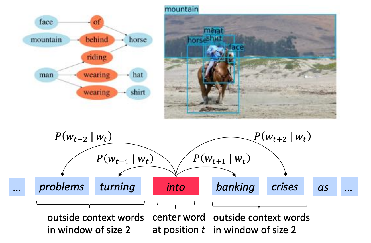 This is a scene graph
We want a graph representation where each node can be an object or an object part and we want to model the spat al or other types of relationship between them, in this case showing that the man is wearing a hat and and the mountain is behind the horse.
This similarly occurs in language, where we may want to model more than just the sequential structure in a particular sentence. We may want to model different interrelationships between the words, for example being able to model which words come across which contexts, or being able to model things like parse trees or grammatical structures.
Relationships are Everywhere
The structures that we want to represent may go even higher level than that. We may want to represent all concepts in the world.
 https://github.com/facebookresearch/PyTorch-BigGraph
This shows a data set called Wikidata, which has elements such as people, places, occupations and so on and maybe even has information about relationships such as a person can be an author. We may want to learn feature vector representations for each nodes in this. For example each element here, each data point might have an associated feature vector representation. And this feature vector should represent the structure in some way. For example, things that are conceptually similar should also be similar or close by in terms of their feature vectors. Maybe we can also explicitly represent this as a graph. That is we can have nodes and edges, where edges represent some sorts of relationships or similarity.
The Space of Architectures
If you think about it, the current architectures we have discussed, fully connected layers and convolution neural networks, cannot really represent these kind of structures. In some case, convolution layers do add architectural biases in terms of connectivities. That is based on our knowledge of computer vision, we add some bias in terms of how nodes are connected to the image. But what we want is something more general, that is a general method to represent relationships between different items, and we want to do this in a learnable way. That is we do not want to impose connectivity patterns for particular domains. We want to just have some representation that can hopefully learn this connectivity pattern, given the particular data and the structure in it.
And so we will talk about various forms of architectural biases that researchers have developed. Ranging from recurrent neural networks, which are typically designed for things like sequential data to more general attention-based mechanisms that can up or downweight a whole range of elements in a set. And this can be an ordered set, such as language, or it can be arbitrary set of different unordered items. And we can generalize this even further to a graph representation, where we explicitly model nodes in this graph and their feature vectors, and then represents the neighborhood of that node and we are able to use that structure to refine the features to represent not just local features, but also features of the neighborhood.
Graph Embeddings
In other words, graphs are the more general way to look at this.
-
Embedding: A learned map from entities to vectors of numbers that encodes similarity:
- We can have embeddings or vectors, for each node - we already know how to do this for images, we feed it through a pre-trained CNN, we can also do this for things like words. In general we can come up with embeddings or vector representations for anything.
- Once we have these embeddings, we can represent them as a graph where the nodes are feature vectors and the edges represent some sort of connectivity or similarity.
-
Graph Embedding: Optimize the objective that connected nodes have more similar embeddings than unconnected nodes via gradient descent.
- For example C we can find the input nodes (A,B in the above graph) that are similar in terms of some type of relationship, and this can be multiple types of edges. For example we can represent in that computer vision image example, something being on top of the horse, or something being in front or behind and these can be different types of edges.
Propagating Information
When representing structured information, several things are important:
-
State: Compactly representing all the data we have processed thus far.
- In the beginning this is just the different nodes or elements that occur in this image. For example the mountain, the man, the horse can all have features associated with them extracted from a CNN and a object detector. So each of these regions of interest have associated features to them.
-
Neighborhoods: What other elements to incorporate?
- We have things like neighborhoods, which represent what other elements to incorporate, these are edges in the graph. For example should a man and a horse be connected for this image, and if so, through what relationship? Typically, we do things like similarity relationships, although in this case, you can also see other things like spatial relationships or verbs that one element is performing on the other.
- Once we have the nodes and the relationships (edges), we can propagate information. What we want to do is represent as a vector the notion that the man is riding a horse. Its not just a man or a horse, it is two interconnected objects and we may want to have a representation vector that represents that relationship.
- Can be seen as selecting from a set of elements
- Typically done with some similarity measure or attention
-
Propagation of information: How to update information given selected elements
- And so what we will do is through the nodes and the edges, perform some functions or computations in the computation graph that combines these different vectors together in a special way that we will see. For example, a weighted summation in order to come up with a new vector that represents not just individual terms but also the items as seen through their relationships. This is essentially a problem of propagating the information.
The above is an example of an image. Similarly, in language you will have a set of words that will read through the document, and we will have a state representation that will track through the sentence. And in that case, it is not a complex graph structure, its just a flat linear sequential structure. But concepts that we will learn actually will relate to all of these different types of forms of structures.
Differentiably Selecting a Vector from a Set
One of the key elements for how to update the representation of a particular node based on its neighborhood, or some other sets of elements is what is called an attention mechanism. And since we want to have a differentiable attention mechanism, typically, we will use things like softmax functions. Specifically, given a set of other vectors that we want to weight up down based on the current node that we are representing, we will essentially do a dot product between our current node and all the other nodes, and then have a softmax function on top of that to convert it to a probability distribution. In that way, you are weighting all the nodes, and and then we will actually compute a weighted summation of all the other nodes and use that to refine this particular node’s representation.
- Given a set of vectors ${u_1,…,u_N}$ and a “query vector $q$,
- We can select the most similar vector to $q$ via $p = softmax(Uq)$
This notion of attention is extremely powerful, because it allows you to represent some arbitrarily sets of information, and this set can be any size. You can apply the softmax function to any sized set, and you can then automatically use that to weight and combine information. And so, again, this can be applied to all manners of structures. this can be applied to sequential structures, where, you are reading a sentence, and translate it to a different language. You can essentially look at arbitrary past words and weight them up and down every time you are converting it to a new word in the target language.
Similarly, you can apply this to graph structure, such that every time you process a node, you can find the weighting or similarity to all its neighbors and use a k-nearest neighbor-type refinement, except in a fully learnable way.
Example: Non-Local Neural Networks
Now we have talked pretty generally about structured representations and relationships between different item. And so, we will make this much more concrete as we move forward and we will talk about specific structures, representations and application such as natural language processing.
However, lets start with a simple example that relates nicely to convolution layers:
If you remember, convolution layers were developed because it did not make sense to connect an output pixel to all input pixels across a high-dimensional image or feature map. This is because we know that we will probably want to extract local features, edges, and so on, and that does not require tying it to the entire set of pixels.
However, we can actually generalize this and allow the network to learn its own connectivity pattern through an attention-like mechanism. This is what is called a non-local neural network. This is called non-local because unlike convolution layers, you do not have for each output node a very specific local receptive field. Instead, what you will have is the equations on the upper as follows:
Specifically, to compute the output $y_i$ - that is the pixel $i$ and the output $y$, we will sum up over all possible inputs g. So this is very similar to a fully connected neural network. Except that inside the summation, we will have a weighted summation, we will have a weighting factor, a multiplication factor, between two functions $f$ and $g$.
\[y_i = \frac{1}{C(x)}\sum_{\forall_j} f(x_i,x_j)g(x_j)\]Now, $g(x_j)$ is just extracting some set of features from the input $x_j$. The function $f$ is a binary function that takes both $x_i,x_j$ because we are computing the output at $y_i$. What we are going is we are going to compute a similarity between $x_i, x_j$ and we are going to modulate the contribution of the features from $x_j$ by that similarity.
- Examples:
- $f(x_i,x_j) = e^{x_i^T x_j}$
- $g(x_j) = W_gx_j$
Specifically for $f(x_i,x_j)$, what we will have is just a Gaussian around the similarity, in this case, just a dot product. A dot product is just an unnormalized cosine similarity. And so what we are doing is we are saying how similar are $x_i$ and $x_j$, and then we are exponentiating. High values means that $x_i$ and $x_j$ are very similar, and low values will mean that they are not that similar. The function $g(x_j)$ is just extracting features, in just a linear way. You just have a $W_g \times x_j$, will be modulated by the similarity function. The output $y_i$ is just the weighted summation across all $j$ and the weighting is dynamically computed based on the data. That is you are computing the similarity function $f(x_k,x_j)$ dynamically.
You might wonder, why is this different from a fully connected layer? The fact that you are doing this dynamically is the key part that makes it different, because when you are doing a fully connected layer, the weights are not dynamic. That is, you learn the weights, and then you apply those weights regardless of the input, they are not data-dependent. In this case, the similarity function $f(x_i,x_j)$ is data-dependent. So you are modulating the inputs in a data-dependent manner, and this makes all the difference.
It allows the network to, in effect, learn the connectivity pattern, learn for each piece of data what is important, and then sum up the contribution across those pieces of data in order to form the output representation.
Here is an example from the paper showing what was learned. This shows arrows across, not just space but also time. One of the interesting things is this summation across j can be not just for the current input, but it can also be the input across time.
And so what we can see is that the arrows with high weights are visualized, whereas all of the connectivity that is ignored is not shown here. And so the red arrows represent high similarity function. What you will want to see if you want to, for example, take a video, which consists of many different frames, and you want to extract what activity is being performed in the video such as playing soccer or kicking, then you allow the neural network to automatically figure out which pixels to pull from across space and time in order to combine those features into an overall representation that at the end, you can use to classify.
Again, this shows the power of attention-based mechanisms to automatically and dynamically in a data-dependent way, figure out what’s important in the input. And it can do this in a way thats not specific to how many there are. If you notice, this function does not actually depend on anything about how many of $x_j$’s we choose from. And so, if you learn this particular neural network, non-local neural network, you can actually apply it to all sorts of other image sizes and so on. This is the power of attention mechanisms in representing relationships between different types of things and we can apply the same type of ideas for representing the relationships between words in a piece of text or between different nodes in a large graph.
Lesson 12: Language Models
Readings
DL Book: Sequential Modeling and Recurrent Neural Networks (RNNs)
Language Modeling: Part 1
Language modeling is the task of determining a probability distribution of a sequence of words, such as the one in the example: $p(\text{“I eat an apple”})$. A language model would also let us compare probabilities between different sequences of words, allowing us to determine which of the two sequences is more likely:
\[p(\text{"I eat an apple"}) > p(\text{"Dromiceiomimus does yoga with T-rex"})\]But still, even assuming we managed to do this with real text, instead of with the silly examples, what would that achieve?
Before we explore real world applications, let us drive abit deeper into how we would mdoel this probabilities mathematically, which will help us motivate the applications.
Let us define the problem abit more rigorously given a sequence s of words, which we can decompose into $w_1, …, w_n$. We are seeking to estimate its probability, We can expand this into a product of many terms, namely the probability of the first word times the probability of the second given the first times the probability of the third, even the first two and so on:
\[\begin{aligned} p(s) &= p(w_1,...,.w_n) \\ &= p(w_1)p(w_2|w_1)p(w_3|w_1,w_2)\dots p(w_n|w_{n-1},\dots,w_1)\\ &= \prod_i p( \underbrace{w_1}_{next word} | \underbrace{w_{i-1}, ..., w_1}_{history}) \end{aligned}\]Note that all is done is to simply apply the chain rule of probability, so this is very general. In other words, all we have is a product of conditional probabilities over the variable $i$, which indexes our words. After the first term which trivially reduces to the probability of the first word, these terms can be interpreted as the probability of the following word given all of the previous words.
The sequential construction helps us see how language models are, infact generative models of language. Indeed, we can easily new sequences of words with it, starting from a history of past words, which could simply be empty, if we are at the beginning of a sentence.
We can repeatedly generate new ones by randomly sampling from the conditional probability of the next word, given the history.
Applications of Language Modeling
- Predictive typing
- In search fields
- For keyboards
- For assisted typing, e.g sentence completion
- Automatic Speech recognition
- How likely is the user to have said
My hair is wetvsMy hairy sweat?
- How likely is the user to have said
- Basic grammar correction
- $p(\text{They’re happy together}) > p(\text{their happy together})$
Conditional Language Models
Standard language Modeling:
\[p(\textbf{s}) = \prod_i p(w_i|w_{i-1},\dots,w_1)\]A related problem - Conditional language modeling, and it is extremely useful and has a ton of applications.
\[p(\textbf{s} | c) = \prod_i p(w_i|c, w_{i-1},\dots,w_1)\]Like a language model, but conditioned on extra context $C$.
Some examples:
- Topic-aware language model: c = the topic, s = text.
- Text summarization: c = a long document, s = its summary
- Machine translation: c = French text, s = English Text
- Image Captioning: c = an image, s = its computation.
- Optical character recognition: c = image of a line, s = its content
- Speech recognition: c = a recording, s = its content
Recurrent Neural Networks: Part 1
RNN is a class of neural architectures which are designed to model sequences.
Why Model Sequences?
- Audio Signal
- Optical Character Recognition (OCR)
- Sentiment analysis
Sequence Modeling
- Many to Many: Speech recognition, OCR
- Many to one: Sentiment analysis, topic classification
- One to many, many to one.
How to feed words to an RNN?
As a first approach, we can just use a one-hot vector representation, where all entries of a vector are zero, except for the entry corresponding to the word’s index, which is one.
Modeling Sequences with MLPs
So how do we build a neural network that can process inputs which are sequences? We can try using a multi layer perception, the input would be the word vectors and we would train the network to perform sentiment analysis.
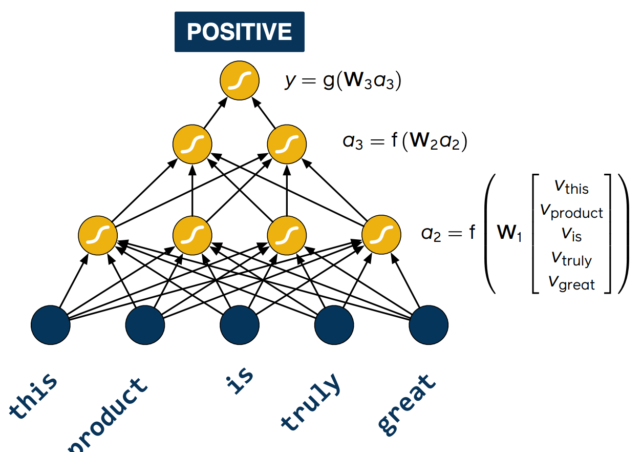
However, we quickly run into problems the moment we try to feed in a different sentence to a network. The sentence here is the wrong length for the network, so what do we do with the words that do not fit?
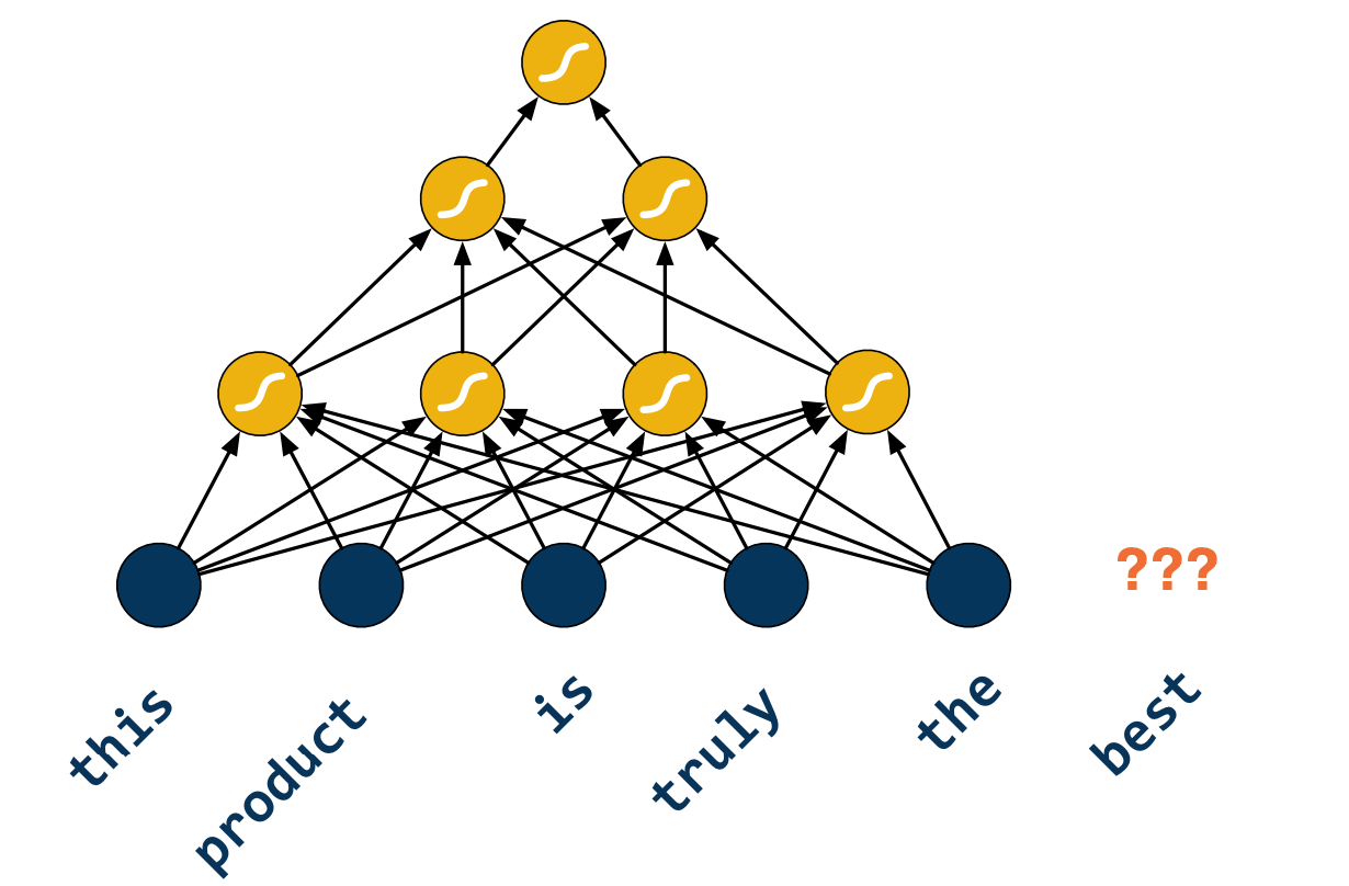
Pain points:
- Cannot easily support variable-sized sequences as inputs or as outputs.
- No inherent temporal structure.
- The order of words matters, e.g a word coming before another word
- No practical way of holding state.
- e.g I am inline at the bank vs I am by the river bank means two different things of the word “Bank”.
- The size of the network grows with the maximum allowed size of the input or output sequences.
Recurrent Neural Networks: Part 2
RNNs are a family of neural architectures which has been designed to model sequences. At every time step they will receive an input and use that to update a state $h_t$. In order to do so, they also have access to the state and the previous time step $h_{t-1}$
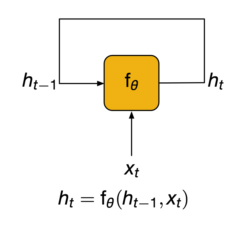
We can draw the arrow a little differently to illustrate the recursive nature of this process. the yellow box $f_\theta$ which we will call the cell gets repeatedly called to update the state. This also explains why these models are called recurrent. Mathematically we can just model this as a function $f_\theta$, where $\theta$ is used to represent the set of training weights of the network.
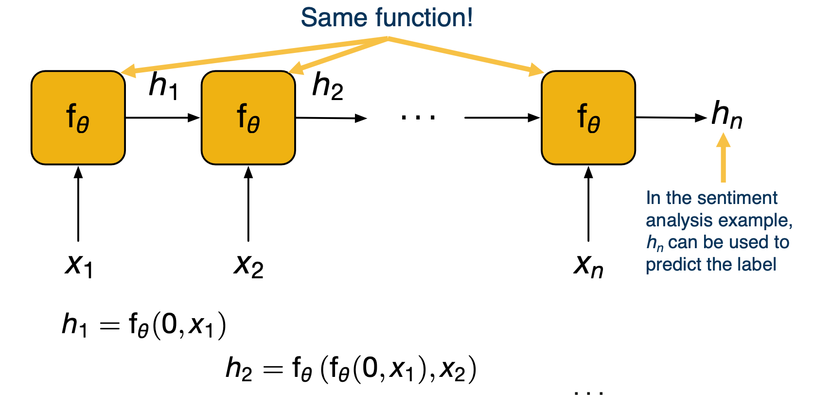
We can expand this picture along the time axis, by unrolling the previous diagrams for n time steps. At time step one, the network receives the first input in the sequence, compute the states and passes that on. At time step two, the state is again updated by looking at both the new input and previous state, and so on until the last time step. Crucially, the function $f_\theta$ that is called repeatedly, it is always the same, giving rise to the recursive nature of RNNs. Going back to our example of sentiment analysis, the final state $h_n$ can be used to predict our label as the network has now seen the whole text.
Backpropagation through time
- Outputs are either directly the states $h_t$ or are computed as a function of those.
- Backpropagation works as normal, by “unrolling” the network (sometimes this is called backporp through time)
- Run the network and compute all the outputs
- Compute the loss (typically a function of all the outputs).
- Perform the backward step to compute gradients
- Can use “truncated backpropagation through time”
- If you have too much history it becomes expensive to backprop.
- The states are carried forever, but we only backpropagate for a fixed number of time steps backward.
“Vanilla” (Elman) RNN
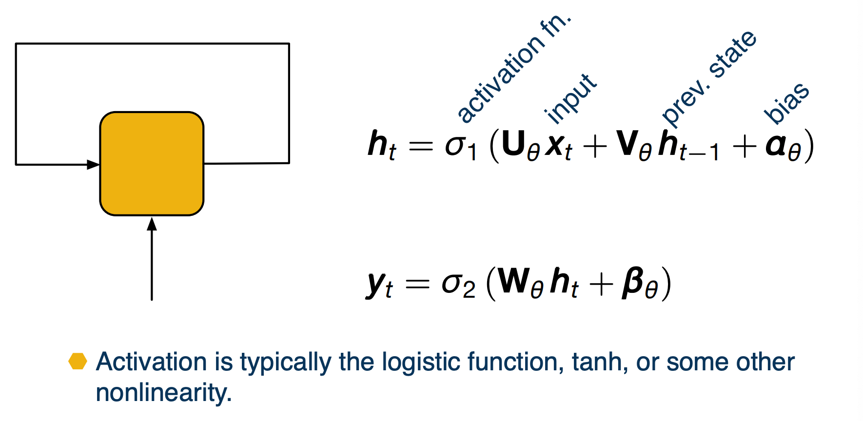
The status update is obtained by performing an offline transformation of the input and the previous state. That is, we multiply the input by a learn matrix, do the same for the state and add a bias term (also learnt).
We then apply an activation function and another affine transformation of this plus an application of a potentially different activation function $\sigma_2$ to get the output. The activations used for these networks are typically the logistic function (also known as sigmoid), or the hyperbolic tangent or some other functions with similar properties.
The term RNN is somewhat used colloquially here without giving a precise definition. The examples have shown you here are what people will commonly understand if you say RNN. Sometimes though the term is also used more formally, to indicate any neural network whose information flow does not follow a directed acyclic graph.
The Vanishing Gradient Problem
RNN in practice can be difficult to train due to a problem known as vanishing gradients.
Let’s discuss this by looking at a simple example:
\[x_t = \sigma(w_\theta x_{t-1})\]Consider this trivial RNN which takes an input at timestamp 0 and then repeatedly updates itself by multiplying its state by learned weights. If we look at the gradient of the state at time t with respect to the state at time 0, we see that this is proportional to the weight $w_\theta^t$
\[\frac{\partial x_t}{\partial x_0 } \propto w_\theta^t\]Now this is a quantity that we have to deal with in the update rule to train this RNN and the power of t is a problem. The reason is that for large T, is the magnitude of $w_\theta$ is greater than one, then the gradient will get very large and the update steps will get erratic. On the other hand, if the magnitude isl ess than one, then the gradients get vanishingly small and the model does not get trained at all.
Long Short-Term Memory (LSTM) Networks
An idea to attempt to alleviate these problems came in the 90s in the form of a different architecture. It is known as the LSTM network or long short term memory network and these are its object roles.
\[\begin{bmatrix} f_t \\ i_t \\ u_t \\ o_t \end{bmatrix} = \begin{bmatrix} \sigma \\ \sigma \\ tanh \\ \sigma \end{bmatrix} \bigg(w_\theta \begin{bmatrix} x_t \\ h_{t-1} \end{bmatrix} + b_\theta \bigg)\]The first four values defined here are the gates and intermediate values:
- $f_t$ forget gate
- $i_t$ input gate
- $u_t$ candidate update
- $o_t$ output gate
The main update rules:
\[\begin{aligned} c_t &= f_t \odot c_{t-1} + i_t \odot u_t \\ h_t &= o_t \odot tanh(c_t) \end{aligned}\]- $c_t$ cell state (new!)
- $h_t$ hidden state
Notice that on top of the state $h_t$ which we already had before, we have an additional cell state $c_t$. This definition is important in avoiding the vanishing gradient problem. Know that it is updated in an additive way by adding something to its previous value $c_{t-1}$. This is different from the multiplicative update rule of RNNs which as we saw got us into trouble.
Also we should note that this is fundamentally different from the element RNN we covered previously, and many RNNs when unrolled are essentially just feed forward neural networks with affine transformations and nonlinearities. Instead, this is completely new. With the idea of gating we are now taking parts of the input to the cell and multiply them together.
To get a better feel for how LSTM works, lets look at how an update is performed step by step.
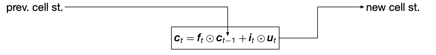
We start with the previous cell state $c_{t-1}$ which is used along with some other values to compute the new cell state $c_t$
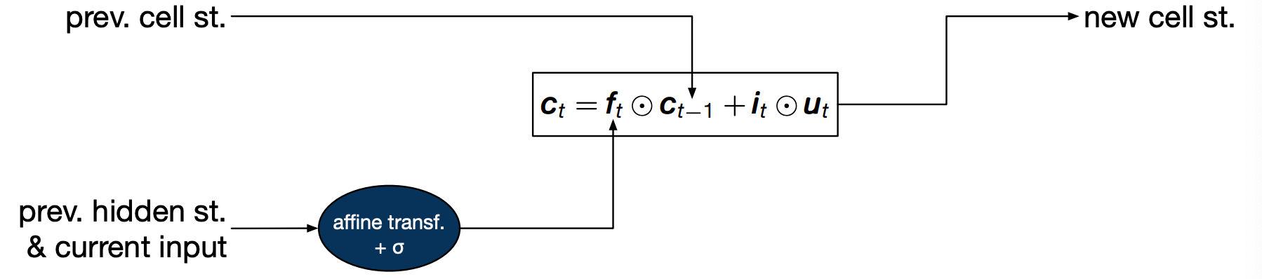
The first value is the forget gate $f_t$ is the result of an affine transformation of the previous hidden state and the current input, pass through a sigmoid so that it lies between zero and one. Intuitively, this gate decides how much of the previous cell state we want to keep around. The two extremes when its value is 0 in which case we forget everything, and when its value is 1, in which case we will remember everything.
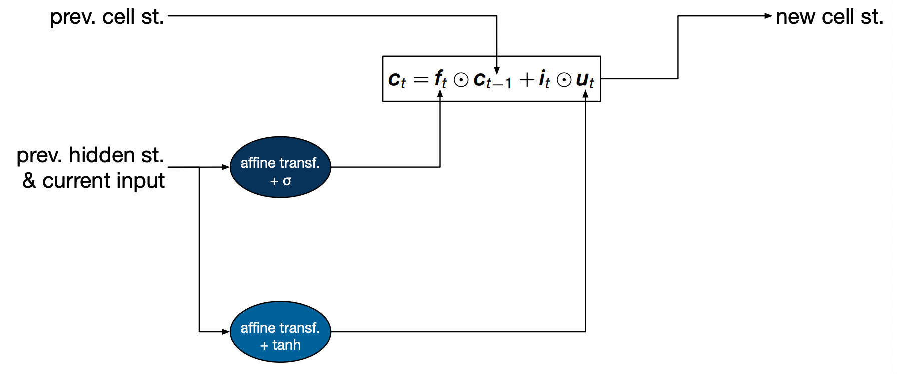
But the old cell state is not all we use to compute the new cell state. We also have a cell called candidate update, $u_t$. Intuitively, this is the new information coming from the input we’ve just seen.
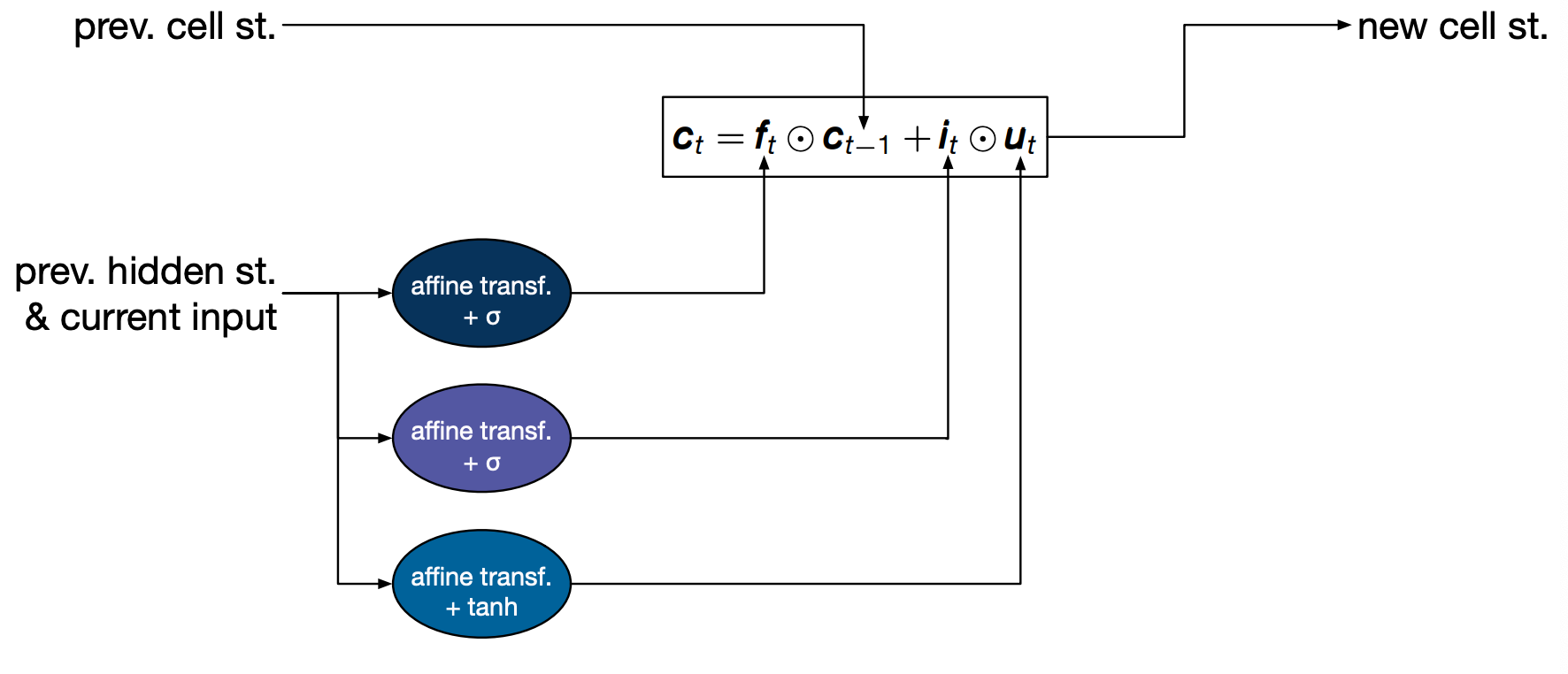
This is also modulated by a gate the input gate $i_t$. Intuitively this decides how much we should let this particular input affect the cell state.
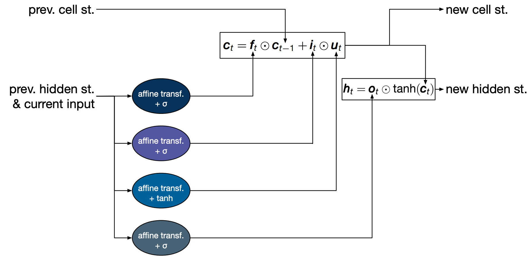
Finally, the update state is used to compute the hidden state, which is the value that can then be used to compute an output. The value of the hidden state is modulated by an output gate $o_t$ which decides how much of the cell state we want to service.
Language Modeling: Part 2
The way a language model would work is as follows, assume that we want compute the probability of a word, given the ones that came before. As we saw previously, the scan of conditional probabilities are central to language modeling. In order to do this, we will input the words in the history one by one, then make use of the output of the RNN at the final time step, to perform a prediction.
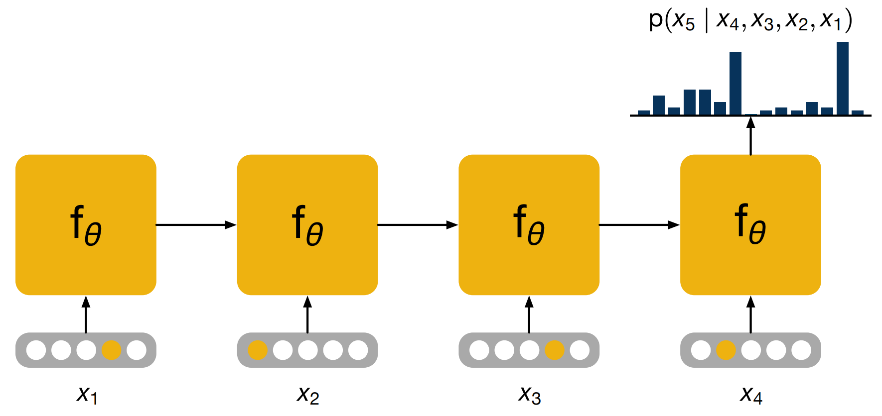
The yellow dots in the inputs are used here to indicate one hot representations which is just one choice of representations.
Let’s look at this process step by step. This is the inference part, that is, we are running the model in forward mode only to perform a prediction, assuming it has already been trained.
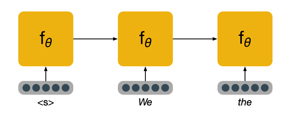
We start with the first word, in the form of a vector representation of a word. In practice, it is often useful to have a special symbol, to be the first word to indicate to the model that a new sentence is starting. We then feed the words in the history until we run out of history and then we take the hidden state age, perform a transformation of it to project it to a very high dimensional space that has the same dimension as the number of words in our vocabulary. And then we normalize this vector using a softmax, which leaves us with a probability distribution of what the model believes could be the next word.
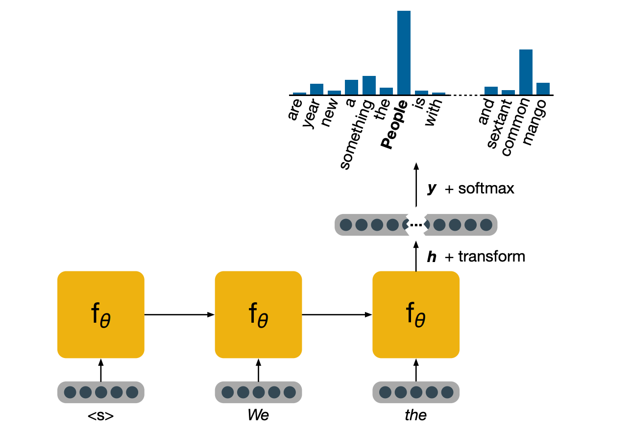
In this case, people is the word that the model feels the most confident about.
Evaluating LM performance
Before we look at training, it is useful to be able to measure how well a model is doing at language modeling. If our model is good, it will assign high probabilities to real sentences. In order to get a measure of performance, we can use a quantity from information known as cross-entropy.
Given a reference distribution $p^*$ and the proposed distribution $p$, cross is defined as:
\[H(p^*,p) = - \sum_{x \in X} p^* (x) log p(x)\]Intuitively, this can be seen as the expected number of bits required to represent an event, drawn from the reference distribution $p^*$, when using a coding scheme optimal for $p$.
Per word cross entropy:
\[H = - \frac{1}{N} \sum_i log p(w_i | w_{i-1}, ...)\]This is the cross entropy averaged over all the words in a sequence. When the reference distribution is the empirical distribution of the words in the sequence. This is commonly used as a loss function, as it is an effective way of measuring how good the model is at estimating probabilities.
Another value that is seen in language modeling is perplexity, and is defined as the geometric mean of the inverse probability of a sequence of words according to the model.
\[\begin{aligned} Perplexity(s) &= \prod_i^N \sqrt[n]{\frac{1}{p(w_i | w_{i-1}, ...)}} \\ &= b^{- \frac{1}{N} \sum_i^N log_b p(w_i|w_{i-1},...)} \end{aligned}\]Note that we can expand this definition by using the law of logarithms, and we see that the exponent is just the per word cross entropy. Perplexity is commonly used as an evaluation metric. The lower the perplexity, the better our model is. Now this formula can look fairly hostile, and talking about geometric means of inverse probabilities isn’t particularly helpful either. So you may find the following intuition useful.
The perplexity of a discrete uniform distribution of a k events is k. So if you flip a coin and asked me to guess, I’ll get it right about half the times and my perplexity there is two. If you throw a fair die and ask me to guess, i’ll get it right 1/6 and my perplexity there is six.
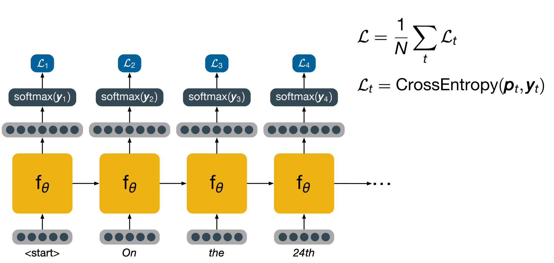
To train a model, we feed the words one by one, using again the special symbol first to indicate the start of a new sequence. After eery time step, we’ve projected a high dimensional space like we did during inference, turn that into a probability distribution and calculate the loss using cross-entropy. Note that at the following time step, that we input into the network is not the word predicted at the previous time step, but the actual word that is present in the training data. This practice is known as teacher forcing and allows the model to keep training effectively even if it would have made a mistake in the previous time steps. Once the whole sentence has been fed, the overall loss is computed as the average of the losses for each word and backpropagation can be used to calculate the values necessary to perform an update step.
Masked Language Models
Intro to Masked language modeling, a task which has been used very effectively in NLP to greatly improve performance in a variety of tasks. You will remember that language models estimate the probability of sequences.
Masked language modeling is a related pre-training task – an auxiliary task, different from the final task we’re really interested in, but which can help us achieve better performance by finding good initial parameters for the model.
By pre-training on masked language modeling before training on our final task, it is usually possible to obtain higher performance than by simply training on the final task.
Masked language models take as input a sequence of words, they add special symbols to mark the start and the end of the sequences similarly to language models.

But they also cover up some of the original words with special tokens that are marked below with the word mask.
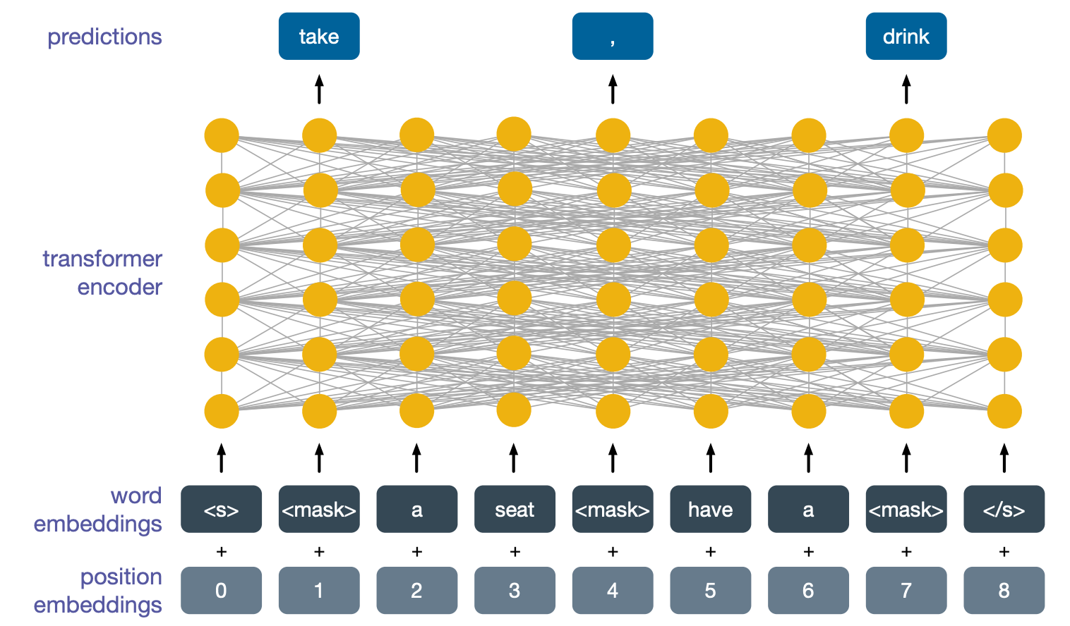
We then take the word embeddings corresponding to these words and we feed them into a transformer encoder. Since transformer encoders have no inherent notion of position of their inputs, and this is useful for language, we also add to the input some special positional embeddings. The final task is to predict what the masked words are. This is abit of a strange and difficult task but it is quite difficult.
A model that learns to solve it well will have not only learned a lot about the structure of language, but also about common sense knowledge. And indeed, this knowledge is quite useful. If we take this model and then train it again to perform some tasks we are actually interested in, the model will not learn to perform the new task but it will also retain part of the knowledge it learned to perform masked language modeling, and this will often give a significant boost in performance. Let’s see how this model can then be trained to perform other tasks.
Token-level Tasks
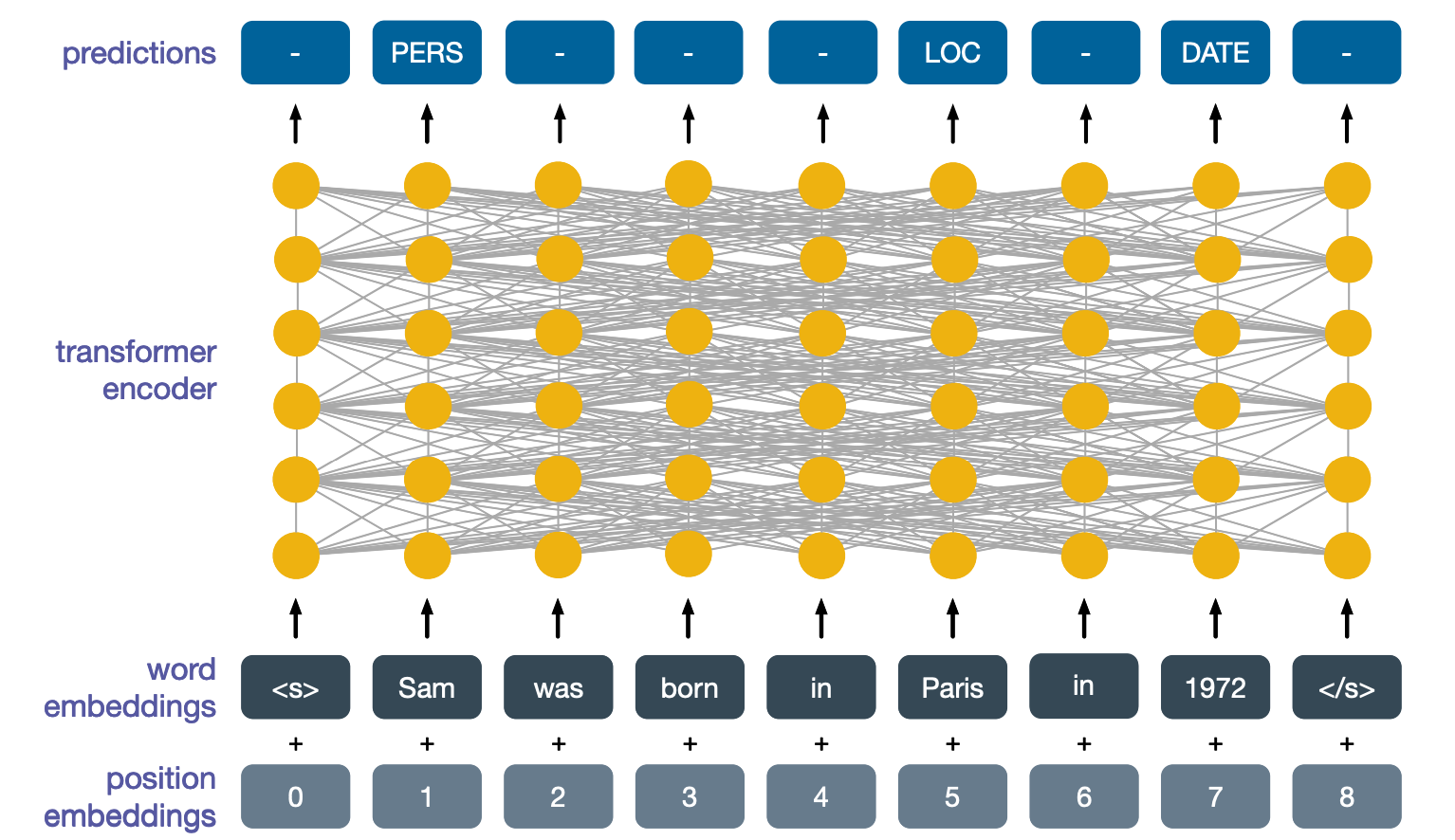
One type of tasks we might want to perform are token-level tasks, where for each output we want to perform a classification. An example is named entity recognition, which involves identifying which input tokens identify entities such as persons, dates, locations and so on. Here we would simply input a sentence without any masked tokens, and for the outputs at each position, we would train the network to perform the correct classification. The labels at the top present the various types of entities, so persons locations, date.
Sentence-level tasks
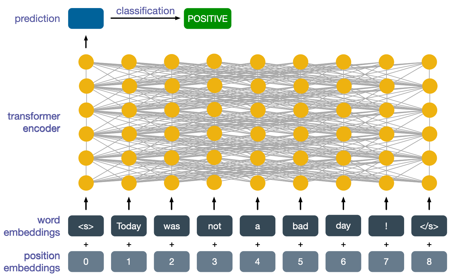
Another type of tasks is sentence-level tasks, where we are more interested in the global meaning of a sentence. An example is sentence classification. Conventionally here we take the first output of the transformer encoder at the top layer and use that to classify the sentence. In this example, we are performing sentiment analysis again.
Cross-lingual Masked Language Modeling
An interesting development of masked language modeling came when people realized that we did not have to stick to a single language. Considering the following two sentences, the first is in english and the second one is its translation in French.
We can join them in a single sequence by using a special separator token and then add start and end special tokens again, and similarly to before, also add masked tokens.
We can then perform masked language modelling of this sequence and the model will learn to look at the two translations simultaneously in order to better predict what the masked words are. Now a model pre-trained with cross-lingual masked language modelling can be used in the same way as a model trained with normal mask language modeling, but the real strength of these models comes from cross-lingual transfer. Imagine we took this pre-trained model and further trained it to perform classification using english training data, because of the cross-lingual nature of its pre-training task, this model would also then be able to perform classification in other languages, even though its training data only covered English.
Cross-lingual Task: Natural Language Inference
Let’s look at another popular cross-lingual task which this model can perform with further training. This is a classic NLP task known as natural language inference (NLI), which we are seeing here and its cross-lingual version. The task is to decide whether the first implies the second one or whether it contradicts it or whether the two sentences are completely unrelated. In this case, the first sentence entails the second one, since if you have had lunch, then you must necessarily have eaten. So far nothing special and this is all monolingual and we are only looking at English data. What makes this interesting is cross-lingual transfer.
So for instance, even if we train the model on a natural language inference dataset that only contain English data, we would find that at inference time the model is also able to work on French data. In this case, the above image depicts the model correctly predicting entailment for these two French sentences, dejeune which means you had lunch, mange implies you ate.
Model Size in Perspective
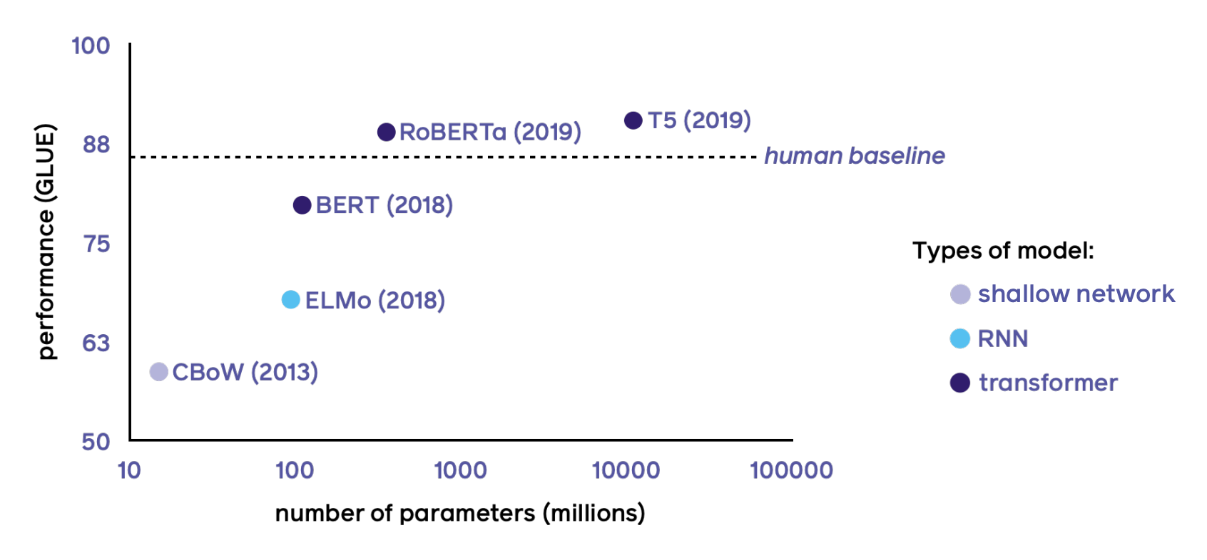
This class of models, which are all based on pre-trained transformers, have been truly revolutionary for NLP. The y-axis is the performance of the GLUE benchmark - GLUE is a set of tasks which are meant to cover aspects of NLP. The nature is not important, and just using it as a proxy for measuring roughly how well a model is at performing language-based tasks on average. The graph shows how well various models perform on GLUE, with the dashed line showing human performance. On the x-axis, is the number of model parameters to give an indication of how large these models are and how expensive they are to run.
As you can see, while transformer-based models have led to an incredible boost in performance, often beating the human baseline, they are also getting incredibly big - and this means they are slower, more expensive to run in terms of computation, memory which leads to higher energy costs and a bigger environmental impact. As an aside, the fact that these models beat the human baseline does not mean much, as these tasks often have very small flaws that machines are very good at exploiting. So while performance on the GLUE task in general is certainly correlated with the ability of a model to understand language, performance relative to the human baseline is not particularly meaningful.
In any case, the problem remains that these models are too big. Fortunately, there are ways to reduce their size while still maintaining most of their performance. Perhaps the most important is known as knowledge distillation.
Knowledge Distillation to Reduce Model Sizes
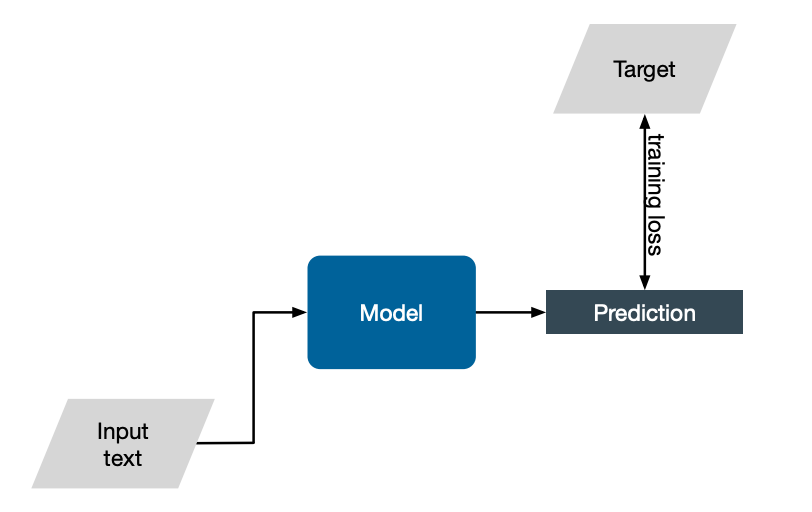
Consider the standard way of training a generic NLP model. We give some input text, the model performs a prediction. We know that the target answer is from the training data, and so we can use a loss function to encourage the model to learn.
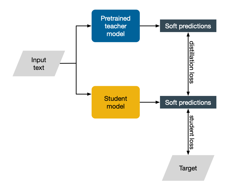
Knowledge distillation works slightly differently. Assume that we have at the top a pre-trained model which we will call the teacher. This model works amazingly well. However it is too slow or expensive to run. We will use this big model to teach a smaller model, which we will call the student. The input text from the training data will be passed to both models and both will make a prediction. Since we know the target that we want the model to predict, we can use a loss like before. We will call this the student loss, as it only involves the student model, and this is just standard training.
Additionally, though, we will also encourage the student model to align its predictions with those of the larger teacher model. Why should this be useful, you might wonder. After all, training using the student loss should provide us with all the training signal we need. Why knowledge distillation works as well as it does is still an open research question. We currently do have some ideas.
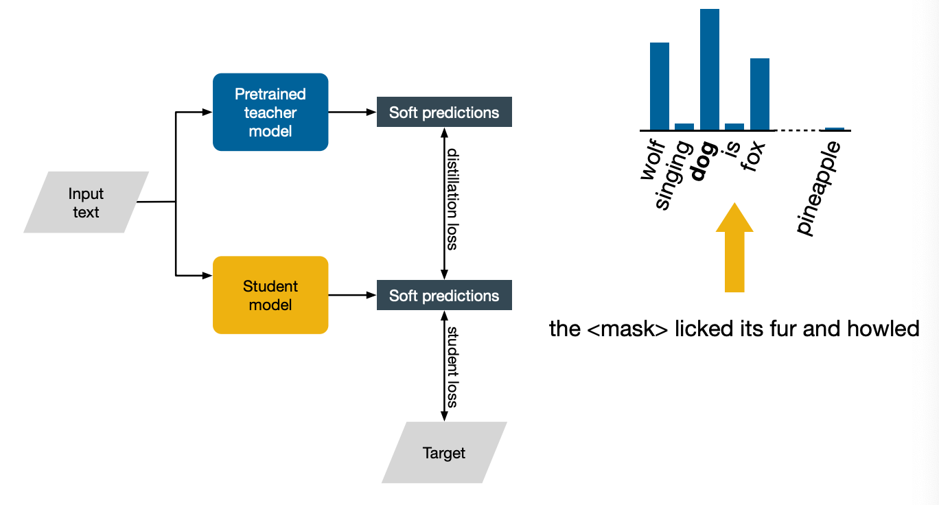
First, notice that the image specifically says soft predictions. ASsume that the task is to predict a word that has been masked. Let’s say that the input sentence is the dog licked its fur and howled, and we mask dog. Now if we look at the predictions made by the teacher model, which has been pre-trained on a lot of text and is very advanced, you will see that it correctly predicts the word dog. The final prediction, the hard prediction, is not the only bit of interesting bits there though.
Notice how wolf and fox also have a fair amount of probability mass, presumably because the teacher model, having been exposed to alot of text, gained some knowledge of the fact that wolves and foxes also lick their fur and also howl. This is why the distillation last between the teacher and the student, which aims to align these probability distributions rather than just the hard predictions, is a useful addition. Instead of just telling us that the right answer is a dog and that’s it, it also tell us that we want to rank wolf and fox highly. And that contains useful information for the student to learn about the world. Another advantage of knowledge distillation compared to just training the student from scratch is that once we have teacher, we can go beyond the labeled training data that we have. We could just take any unlabeled text and use the teacher to make predictions on it, which can then be used to augment the training for the student.
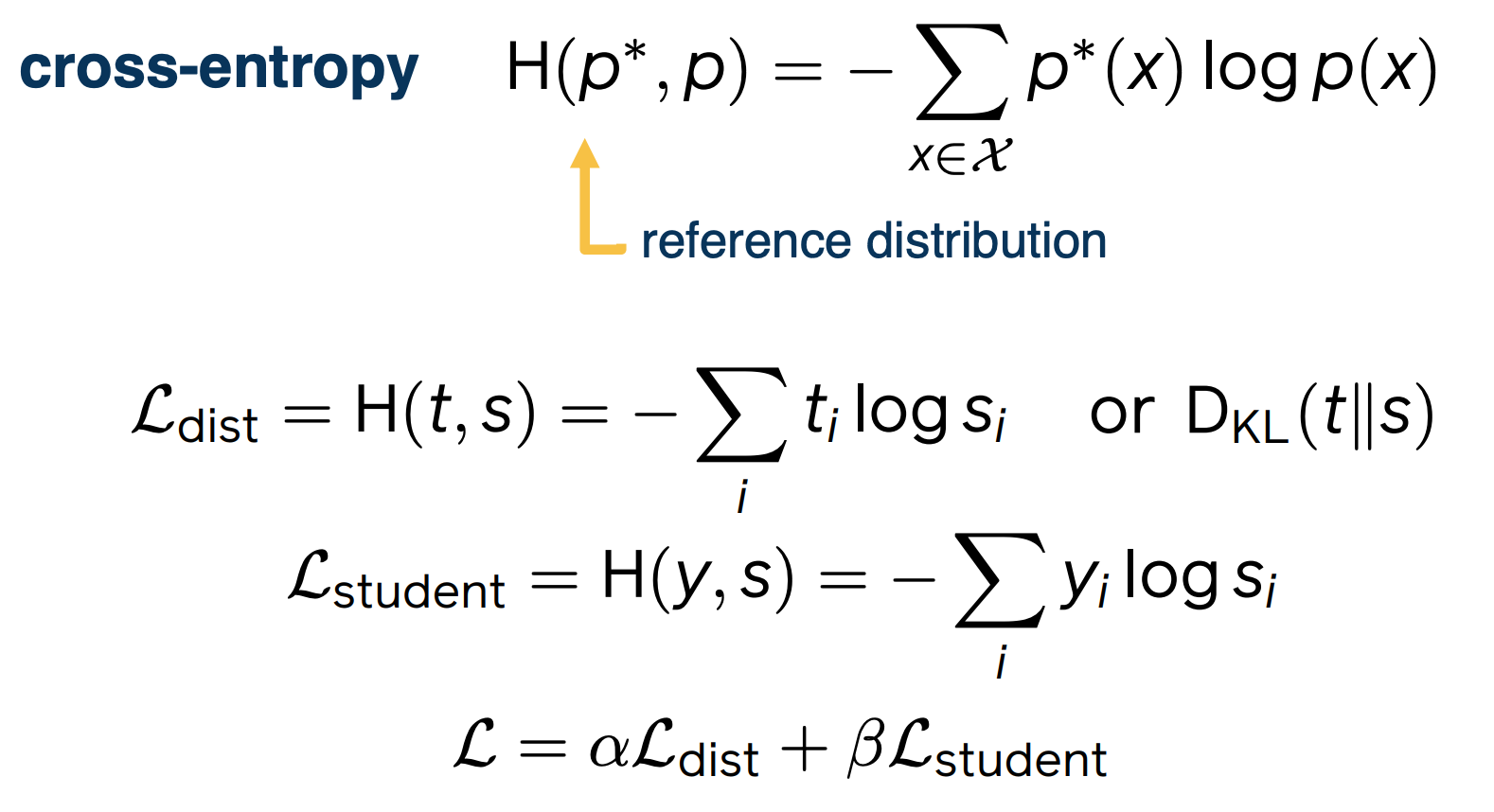
Now let’s look concretely at what the distillation loss would be like for a classifier. Recall that cross-entropy H when talking about evaluating language models. Now, the cross-entropy between two distributions takes its minimum value when the two distributions are the same. For this reason, it is often used as a loss function for distillation, where the aim is to bring as close as possible the target and student models’ predictive distributions. So then for a given example for which the teacher has predictive distribution $t$ and the student model $s$, the distillation loss is simply the cross-entropy between them.
The other common loss function here is the very closely related KL divergence $D_{KL} (t\lvert \lvert s)$. For the other term of the loss, the student loss, this would just be a classification loss. A standard choice here would be again the cross-entropy loss. Although this time, it would be between the empirical distribution y, which is just one for the true label and zero everywhere else, and the student model’s predictive distribution s. For the total loss, this is simply given by a linear combination of these two terms.
Lesson 13: Embeddings
Readings
Embeddings Introduction
- Word embeddings
- Can be used as the initialization of lookup table in LSTM.
- Graph embeddings
- A generalization of words embeddings.
- Applications, word2vec, including ranking, recommendation, classification, and tagging
- Can we actually embed everything? E.g piece of content, relationships etc.
Introduction to Embeddings
In a nutshell, embeddings can be viewed as mapping objects to vectors through a trainable function.
For example, in CNN where it maps an image into a vector in real space. We can also map other things such as text into a vector. Typically the neural net can be seen in RNN or a transformer for text, or simply a shallow one, such as word2vec.
Above is a picture illustrating mapping different objects into the same space. Usually the distance between the vectors in the space is used as a similarity function for different objects. For instance, we want to map similar objects closer in the space. In this case, at the upper right, there is a video about a birthday cake and then it is mapped to close to the text happybirthday and hashtag iamold.
We will be talking about how we are going to learn the vectors of different objects. You will have an idea of what are word embeddings and graph embeddings and how they are learned. You will also learn to use those embeddings in applications and what kind of tasks can benefit from it such as recommendation, tagging, search, etc. You will also get an idea of how large scale computing words for learning embeddings.
Word Embeddings
The search for good representation of words has been a long term pursue in NLP.
-
Distributional semantics: A word’s meaning is given by the words that frequently appear close-by
- “You shall know a word by the company it keeps” (J.R.Firth 1957:11)
- One of the most successful ideas of modern statistical NLP!
- When a word w appears in a text, its context is the set of words that appear nearby (within a fixed-size window).
- Use the many contexts of w to build up a representation of w.
For example, looking at the word banking:
- Government debt problems turn into
bankingcrises as happened - Saying that europe needs unified
bankingregulation to replace the hodgepodge - India has just given its
bankingsystem a shot in the arm…
Natural word Embeddings
There is a series of work based on idea of learning word representations using neural networks. The work proposed by Bengio in 2003, a neuro probabilistic language model proposes the following. It associated h word in the vocabulary a distribution word feature vector. It uses a neural network model essentially tried to predict the next word.
And later the work by Ronarld Collobert and Jason Weston and other collaborators using convolution neural net to know word embeddings. The word word vectors and other parameters of the neural nets is chained on several different asks including language model entity recognition, and part of speech tag accenture was sharing the word vectors and it showed that it is useful for all these tasks. And they also looked at the nearest neighbor of the word vectors and find that it displays the same tactic and semantic properties of words.
More recently, Thomas Mikolov proposed a relatively simple model called word2vec, which is really efficient to compute, where the word vectors are the only parameters to be known in the model because of its efficiency in powerful performances, it gets wider adoptions in both NLP Research and applications.
Collobert & Western vectors
The idea comes from that a word and its context is a positive training example and a random word in the sample context gives a negative example.
So, in this example, the positive example is the phase “cat chills on a mat” and if we take a random word “Ohio”, the negative example becomes “cat chills Ohio a mat”, obviously that doesn’t make much sense. Then the score is calculated by the neural network built on top of the word word vectors, and we want to penalize the score of “chat chills Ohio a mat” and optimize the score of a “cat chills on a mat”, the positive example.
So here we use a margin loss on it, this is similar to the ideas in support vector machine where you want to increase the margin between the positive and negative examples. Is also notice both that we only need positive examples in the training and negative examples are drawn from random words, so in this case, a random word from the dictionary. In the later part of the lecture we will talk more about finding negative samples or negative sampling as it plays a very important role in different embedding models.
Word2vec: The skip-gram model
The idea is to use words to predict the context words. This is the skip gram model, there is also the continuous bag of words model in word2vec which will not be covered.
The context is a fixed window of size $2m$, lets take a look at this following example:
Here is the example the context window is size 2 and we’ll have part of the sentence as problems turn into banking crisis. ASsuming the word “into” is the center word, so we hope to use the vector representation of the word “into” to predict, what would be the context in “into”.
We are trying to make those predictions and change the vector representations in a way that we can do the prediction better.
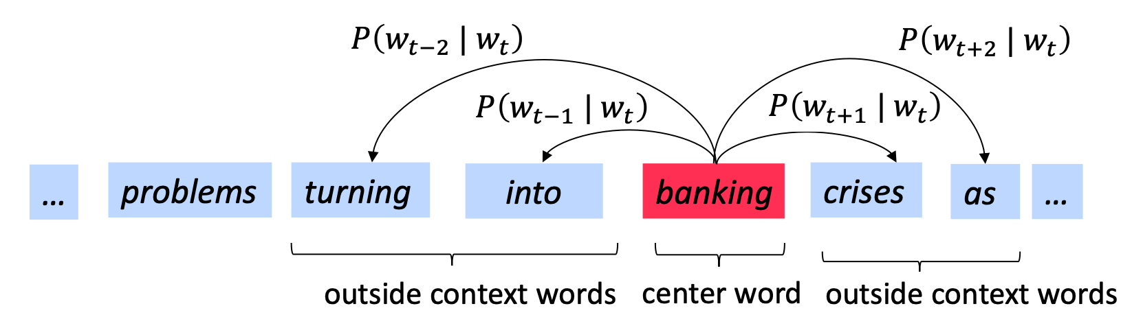
Similarly, we go on to the next word banking and essentially would do the same thing.
More formally, we write in the following formula a skip gram objective function. For each position T predicting the context word within a window of fixed size M, given a central word $w_j$, we multiply all those probabilities to be our likelihood. And here $\theta$ is all the parameters to be optimized.
\[L(\theta) = \prod_{t=1}^T \prod_{-m \leq j \leq m, j\neq 0} p(w_{t+j} | w_t ; \theta)\]The objective function is the (average) negative log likelihood:
\[J(\theta) = \frac{1}{T} log L(\theta) = - \frac{1}{T} \sum_{t=1}^T \sum_{-m \leq j \leq m, j\neq 0} log p(w_{t+j} | w_t ; \theta)\]Notice that in this particular model, the parameters to optimize are only the word vectors and this is simpler than the earlier neural net models and also enables very fast computation.
The question then becomes how to calculate the probability $p(w_{t+j}\lvert w_t;\theta)$. In the word2vec model:
- We have two sets of vectors for each word in vocabulary:
- $u_w$ when $w$ is the center word
- $v_o$ when $o$ is the context word
- Use inner product $(u_w,v_o)$ to measure how likely $w$ appears with context word $o$
\(p(w_{t+j}|w_t) = \frac{exp(u_{w_t} \cdot v_{w_{t+j}})}{\sum_{k\in V} exp(u_{w_t} \cdot v_k)}\)
- This is the softmax!
- $\theta = \{u_k\},\{v_k\}$ are all the parameters in the model!
So we can do stochastic gradient descent on softmax function but the problem is that it is very expensive to compute because the size of vocabulary is very big, making it impossible to compute.
There are two solutions to this problem:
- Hierarchical softmax
- Negative sampling
Other word embeddings
There are other family of word embeddings which also have been widely used. They differ in several aspects such as algorithms, text corpora, dimensions etc. For instance GloVe where the training of the embedding is performed on aggregated global word co-occurrence statistics from a corpus and fastText which is also from facebook AI and has wide adoptions. It adds some more information in addition to word2vec, which better handles auto vocabulary words and it is also available in more than 200 different languages. It is shown to be very efficient for text classification tasks, so you can find pertained word vectors weights below, and a common way of using the embeddings is to use it as features in downstream ML models, or as initialization of neural net models for NLP such as RNN, LSTM. Finally more recently the context tries the word embedding has becoming very popular such as ELMo and BERT, which will be covered in detail in later lectures.
How to evaluate word embeddings?
There are mainly two categories of evaluations, namely:
- Intrinsic
- Evaluation on a specific/intermediate subtask
- Such as taking the nearest neighbor of a particular word or vector
- Fast to compute
- Can check quality of word embeddings during training
- Helps to understand the system
- Not clear if really helpful unless correlation to real task is established
- Evaluation on a specific/intermediate subtask
- Extrinsic
- Evaluation on real task (i.e text classification)
- Can take a long time to compute
- Unclear if the subsystem is the problem or its interaction
- If replacing exactly one subsystem with another improves accuracy $\rightarrow$ (Winning)
- Also use this approach to evaluate other embeddings such as graph embeddings
One interesting example of intrinsic word embedding is the word analogy task.
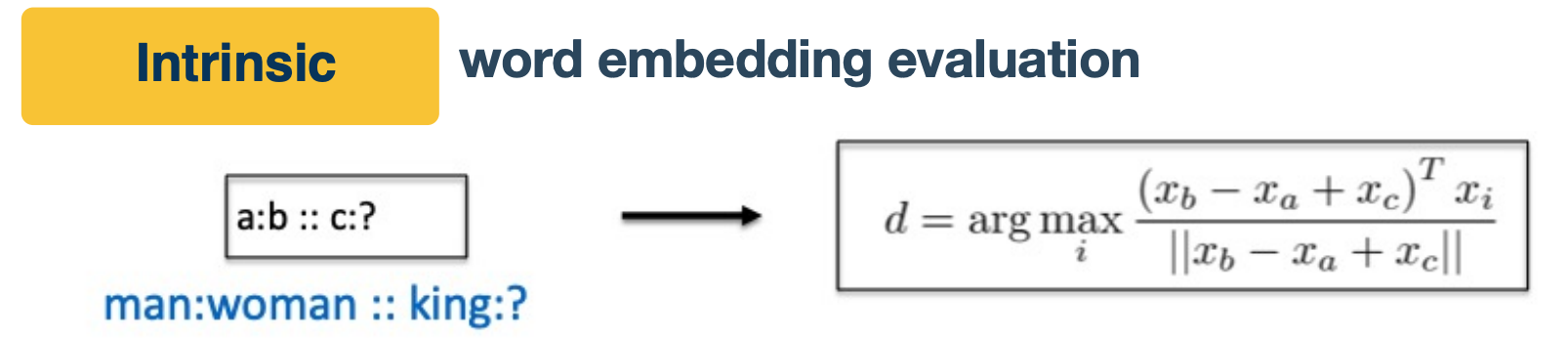
In this task, we have a pair of words, man and woman and the word king. We wanted to know which word to king has the same relation to men to women to men. We observe that the train word embeddings have the following property:
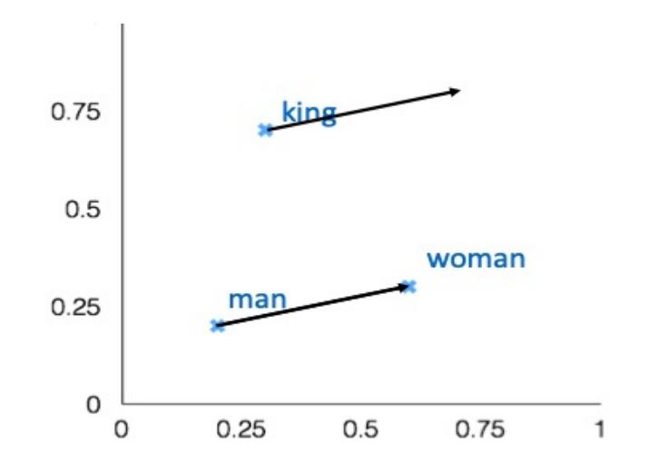
- Evaluate word vectors by how well their cosine distance after addition captures intuitive semantic and syntactic analogy questions
- If you find that the vector satisfy the formula on the top you will find the vector as queen. ( King - man + woman = Queen )
- More examples: http://download.tensorflow.org/data/questions-words.txt
We will talk about Extrinsic in the later sections.
Graph Embeddings
Graphs are networks of entities and connections between them. They can be used to present stuff like protein structures or map data or networks of people’s interactions. Multi relation graph embeddings are typically studied in the context of knowledge graphs.
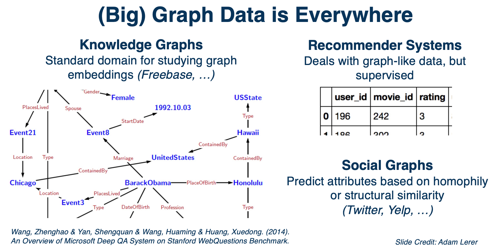
So you can have these graphs structured wikipedia data, and there are other similar graphs like word ontologies. There are also related areas of study such as a recommender system and embedding methods like Deep Work that were primarily designed to operate on social graphs. From previous section we talked about word embeddings, and you can think of it as defining a graph where each word to be a node and the node has an edge to its context word in sentences. And word embedding models like Word2vec are essentially learning the embeddings of the graph node, which is the word.
Graph Embedding and Matrix Completion
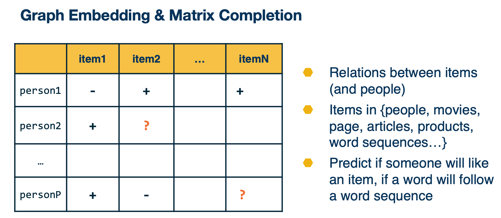
Let’s take a look at an example here. This is also known as matrix completion, where you have a big matrix and you know some neighbors, labels, between persons and items. For instance you know that person one likes item two and do not like item one. There are also missing entires in the matrix, whether there are relations between items and people, and the items can be people, movies, pages, products, word sequences, and you like to predict if someone likes an item or a word, or follow a word sequence.
So you can know the vector representation of people and items here such that some simple form of the function between these two vectors will fit the existing value in the matrix and predicting the unknowns. So that is a particular case that we want to use graphing embeddings for.
Why Graph Embeddings?
We define embeddings as a learned map from entities to vectors of numbers that encodes similarity. A mapping is just an algorithm that convert entities with relations to vectors or features that include similarities. For word embeddings, you enter features such that the features of a word is similar to the features of the words surrounding it.
For graph embeddings, you enter features that connected nodes are more similar than unconnected nodes and enter these embeddings by optimizing this objective by stochasic gradient descent. In other words we are talking about graph node embeddings here, and note that you can also do path embedding in the graph structure embedding which will not be covered.
Just as word embeddings, graph embeddings are a form of unsupervised learning on graphs. It can be used as task agnostic entity representations. The features are useful on downstream tasks without much data. And the nearest neighbors are semantically meaningful.
One family of graph embeddings
This is from the open source project pytorch BigGraph where several graph embeddings were implemented in a large scale setting. Here we are going to talk about a family of graph embeddings that we spurred in PyTorch BigGraph and essentially the way we trained those embeddings.
So given that we have a multi relation graph like the one below, where different colors of the edge representing different relations, we want to optimize the loss function L such that for a simple function of an edge e, and a negative sampled edge, $e’$, we want to minimize the margin loss as similar to the loss in the Collobert & Western vectors.
Margin loss between the score for an edge $f(e)$ and a negative sampled edge $f(e’)$:
\[L - \sum_{e \in G} \sum_{e' \in S'_e} max (f(e) - f(e') + \lambda , 0)\]The score for an edge is a similarity (e.g. dot product) between the source embedding and a transformed version of the destination embedding, e.g.
\[f(e) = cos(\theta_s, \theta_r + \theta_d)\]- $\theta_s$ is the source, $\theta_r$ relation vector and $\theta_d$ is the destination node vector.
Negative samples are constructed by taking a real edge and replacing the source or destination with a random node
\[S'_e = \{(s',r,d) \lvert s' \in V \} \cup \{ s,r,d' \lvert d' \in V \}\]Let’s take a particular edge here as the edge b to c. So essentially the loss function is saying that we want the distance between the vector b and the transformed vector of c to be close and the distance between vector b and transformed vector of a and e to be large as there is no edge between them.
Similarly we do this again for positive edge b to c and negative edges a to c and d to c. So the loss can be again optimized by $S_{dge}$, and this is how the graph node embeddings and parameters of the relation’s transformations learned.
Multiple Relations in Graphs
So here are the different types of relations that we spurred in PyTorch Biggraph.
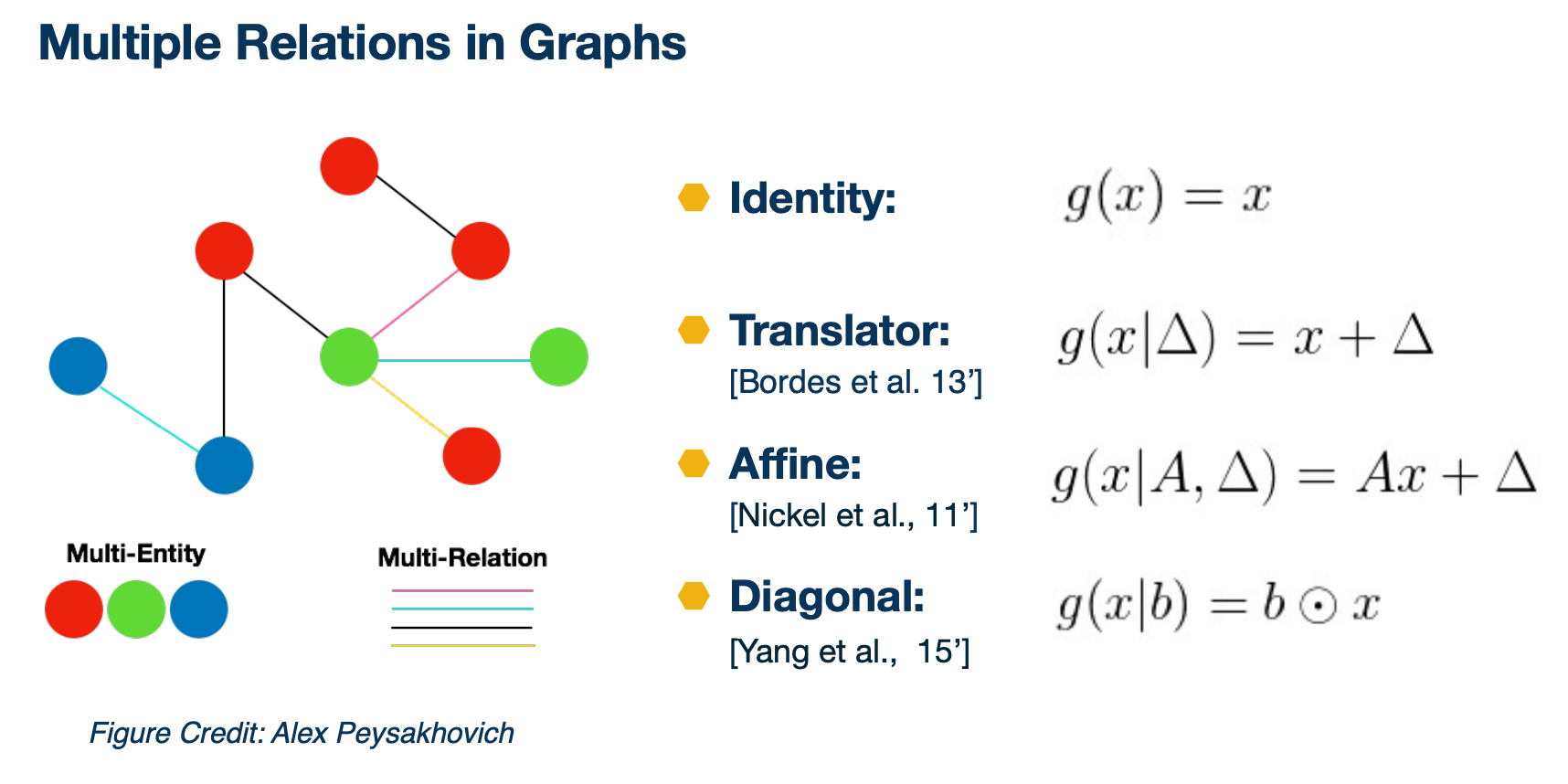
The first one is the identity where we treat every edge to be the same. The second one is a translator where we use a vector to represent a particular edge type and then we add the edge type vector to the node vector. So we can also do a fine translation where we have a matrix A and a translator vector delta for each edge type, and we do multiplication of the matrix A and node vector plus this translator, where it allows more complicated transformation than the translator model. It also has more parameters to be learned. And then we could also have the diagonal transformation, where we have a vector b edge type and we multiply each dimension of b with the corresponding dimension of x.
Embedding a knowledge base
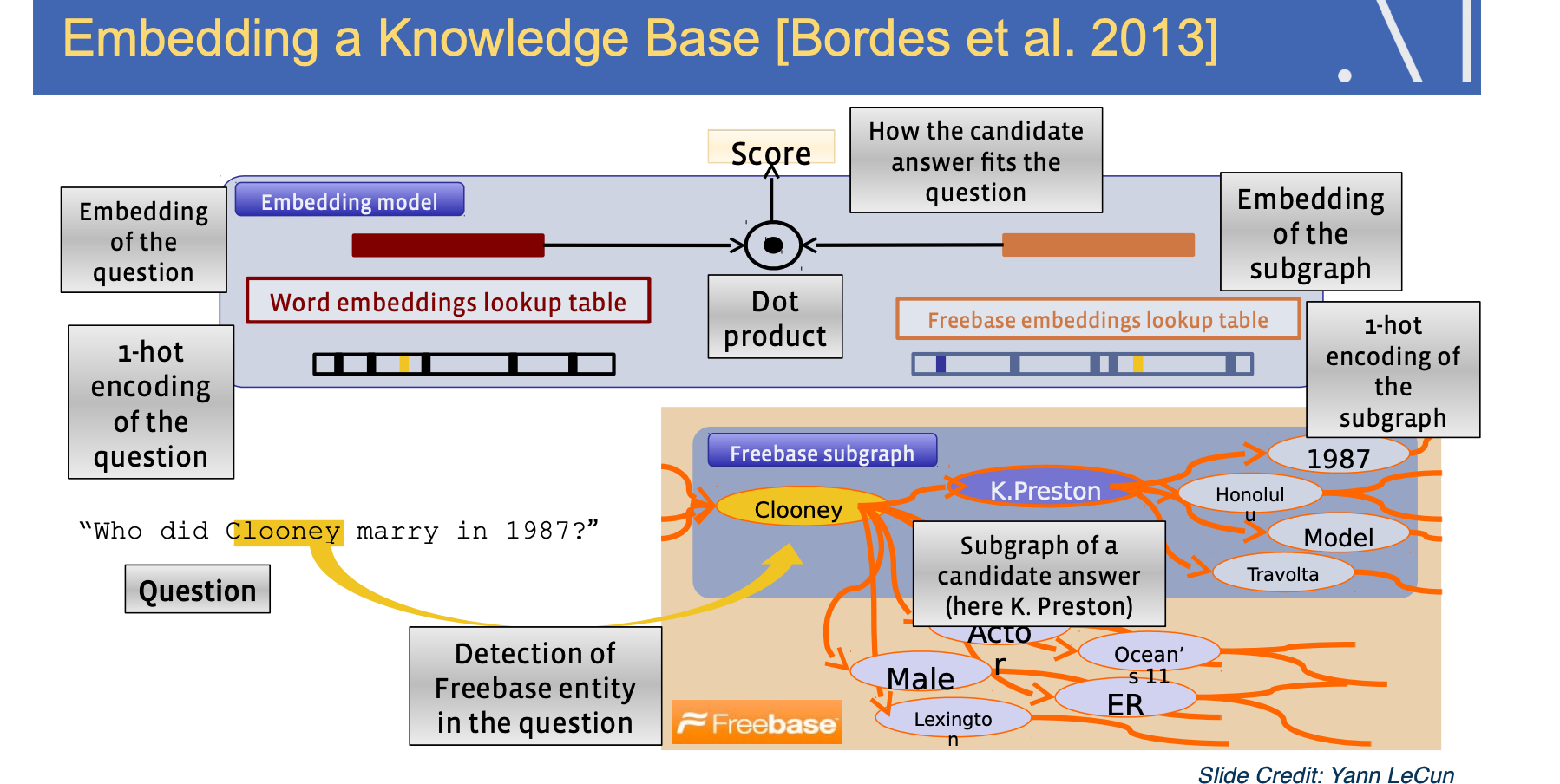
Here is an example from embedding a knowledge base. So we have a subgraph from Freebase, where it has the entities like CLooney, actor, male, and the relations between the entities. We can enter a graph embedding on the knowledge graph, then for question like “who did Clooney marry in 1987” you also have embeddings of the question through the word embedding table. You can then detect the entity in the question and find the corresponding entity in the freebase subgraph and to find the relevant entity to answer for this question through entity embeddings, so that is the high level idea.
We are going to talk more about examples of how to use graph embeddings in the applications section.
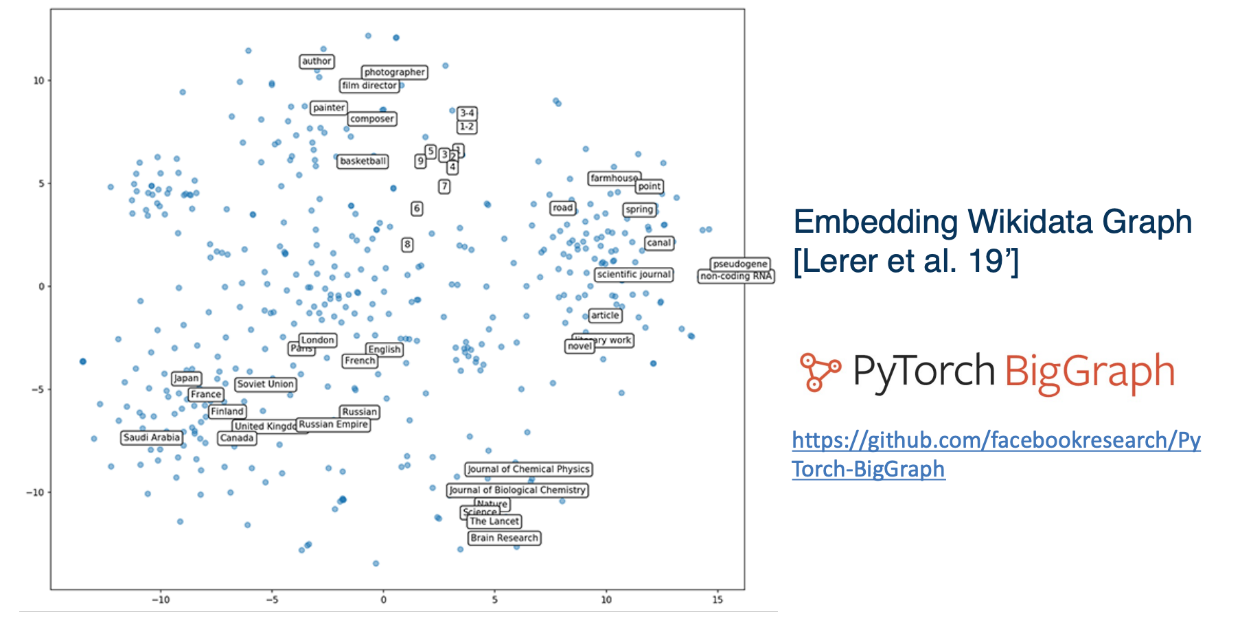
Let’s take a look at two dimensional disney visualization of the entire wikipedia graph from the pytorch biggraph project. So we follow the method in transient, but we scale it to 55 mini entities in 3 billion edges with 5000 different relations.
This picture above is the visualization of the top 500 popular entities on wikidata projected in two dimensions. There are several clusters which is quite meaningful. For instance the lumbers are clustered together and from the top cluster in the middle you can see different occupations. And there is a cluster of countries on the left bottom and the entity embeddings learn on the knowledge graph exhibit certain behaviors in the vector space and you can usually find meaningful clusters. We will see those properties again in the application section.
Optimized Negative Sampling
So in order to train embeddings fast on a giant graph like wikidata, we need to optimize alot of things.
One thing that is particularly helpful is that we called optimized negative sampling. Recall that in the previous section that we are talking about sampling negative nodes to construct fake edges, but the training time is dominated by computing the scores for fake edges. But how can we speed that up? So what if we cropped a sub batch of 100 edges with the same set of random nodes. In other words when you do like batch training, you use the same set of hundred edges without redoing the sampling. This obviously reduces random access memory bandwidth by 100x, and if the similarity matrix is dot product, a batch of negative scores can be computed as a matrix multiplication and that could further help in efficiency. We find this trick to be really useful in practice and the graph above shows how you can increase the number of edges present per second with doing batch and negatives comparing doing unbatched negatives. We also build techniques to enable distributed training for graph embeddings. That further enables us to train really giant graph embeddings.
Applications, world2vec
- TagSpace
- Input: Restaurant has great food
- Label: #yum, #restaurant
- Use-cases - You wanted to inquire proper hashtags for tags without hashtags. So this is quite similar in the word embedding case. You can have edges between words and hashtags, given those words and hashtags appear in the same post and learn embeddings for both of them, then oyu can use the embeddings to:
- Labeling posts
- Clustering of hashtags
- PageSpace
- Input: (user,page) pairs
- Use-cases
- Clustering of pages
- Recommending pages to users
PageSpace
HEre is a example of news and page embeddings. If we search for nearest neighbor for the page, the new york times, we can get pages such as washington posts, bloomberg politics. They are all close in the embedding space. Obviously, we can use it to recommend users who follow the new york times other similar pages.
From practical point of view, how do you search the nearest neighbors best efficiency from millions, billions of vectors is a very important issue. So for this we use faiss, a library for efficient similarity search and cost sharing both dense vectors. Now we only use the users engagement data or behavioral data for learning the page embeddings, we have not use any content information yet. So for instance the title and description of the page often tell you a lot and images or videos on the page is also informative.
VideoSpace
In the example of videospace, we started considering more relations information in the graph. We have pages, which published videos. The video contains words in its title and description and we also have visual content. We also know information about the video, for instance certain users have engaged with the video and we have human labels on the topics and subtopics of the video. Now we would like to get a representation of the video by the following:
First, for pages we have a giant lookup table initialized with the trained page embeddings. Similarly we also have a word lookup table and word embeddings and we aggregate all the words in the title and description as the text representation. For visual content we took snapshots of video as images and fitted into a classic visual model such as CNN, and use the last layer of each image as the visual embedding. Finally, the embedding features are fed into MLP with other features on top. Now if we use it for classification such as to predict the topic of the video, we add softmax for multi classes classification and if we use it for recommendation, we use ranking loss as similar in the pagespace case where it good at capturing precious information. The entire system is trained end to end with stochastic gradient descent.
So from the video space example, we already seen that different behavioral data and content data is helpful for a bunch of tasks. So what about hte idea that we just embed everything into a vector space? So this leads to the idea of world2vec. Where world is everything in the graph. ng and we want to embed them into vector representations. so here is a simplified version of world2vec where we have the graph. In the center we have users engaging with pages groups and posts and pags can create posts and links from different domains, and so on. So again, this graph is huge, especially if you want to embed a power user in the graph. Embedding all these different entities in single space is pretty powerful. Because you can say things like, which topic is the user interested in? Or which topic does this post belong to? We can also use these embeddings for some other tasks that has very little labeled data like suppose you have a list of 10 videos that in French and want to find more videos in French.

Here is an example of behavior data. IF we can take this behavioral graph and convert it into features that describes the similarity of all these entities based on their interactions, we can use traditional machine learning systems to answer lots of important questions, such as what pages or topics might you be interested in? Which posts contain misinformation, hate speech, election interference? Is this person’s account fake or hijacked? And what songs might you like and even if you have never provided any song information before.
 example of visualization of the embeddings, where the green nodes are misinformation without knowing that it is misinformation
- users
- Bad Actor Cluster
- groups
- ‘for sale’ group prediction
- pages
- recommendation
- page category prediction
- identify spam / hateful pages
- domains
- domain type prediction
- Identify mis-information
world2vec
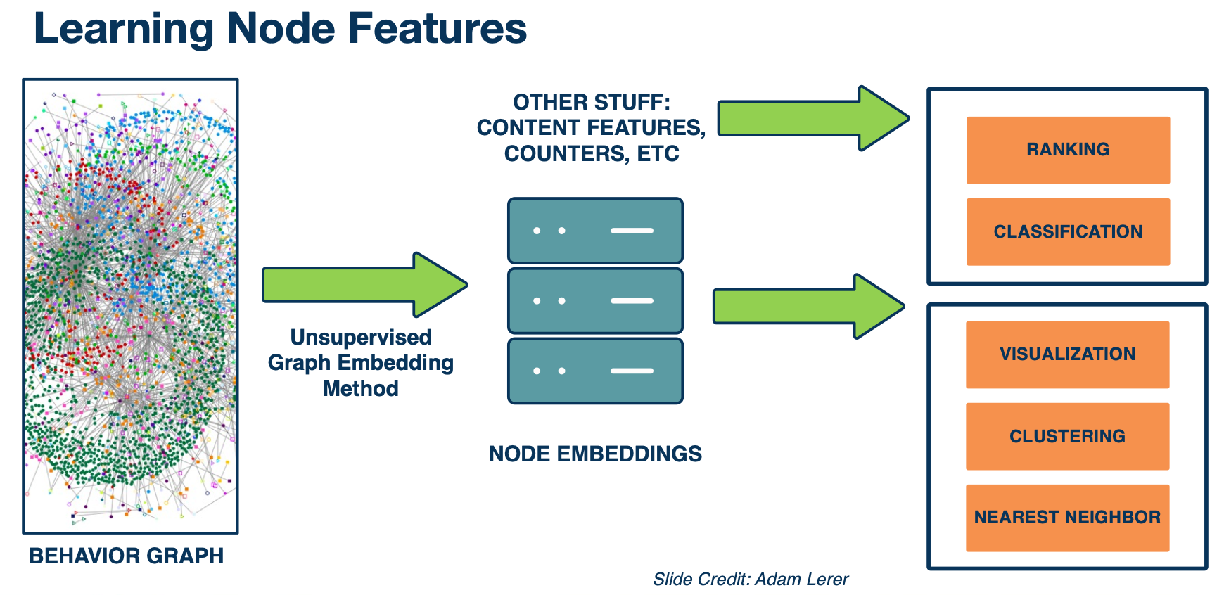
Here is a summary of world2vec. We take a giant behavior graph of different types of entities and different types of interactions between them. We use unsupervised graphing embedding to convert them to node embeddings. Then possibly we combine them with other features such as content features, counters etc. Then we use it for all kinds of different kinds of downstream tasks such as ranking, classification, clustering, finding nearest neighbors and so on.
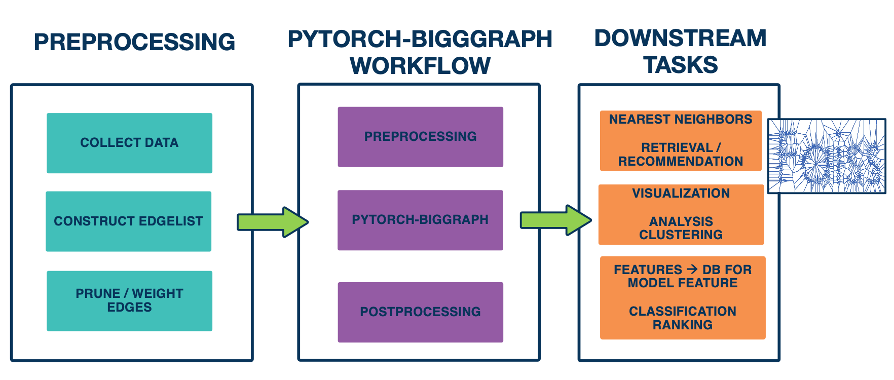
Let’s dive in a bit deeper in technical details. We released the platform we used to train world2vec, which is the pytorch big graph library mentioned earlier. Now let’s go to the overall workflow of training a giant graph embedding model. As the first step, you need to prepare the line graph, that is going to be a list of ideas of the source , destination, and relation types. Then you fit into the pytorch-biggraph workflow, which does some pre processing in the database to shared everything then you run the pytorch-biggraph and then do some post processing.
so you end up with a database table of IDs and their embeddings, which you can use in all different ways as mentioned above. For example, people use it a lot to look for nearest neighbors, so this support very large scale computations.
Here are some techniques on how to scale the graph embedding training algorithms to handle really bigger graphs.
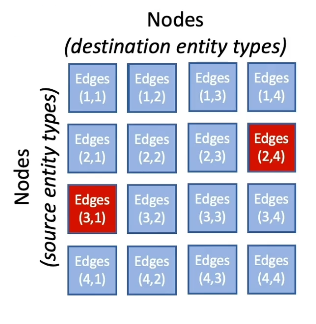
The key idea is to partition the graph, we use matrix blocking to subdivide the graph. First we divide the nodes uniformly into N shards and then according to show the nodes are divided, the edges between the nodes are divided into $N^2$ buckets by the source and destination node.
So the benefit of partitioning the graph into smaller chunks is that we could handle one chunk at a time. In the single machine training, we only take one bucket of edges and then train on those edges. So only two partitions of the model are held in memory and others are swept to disk. This could save alot of memory usage and allows it to train really big models.
In the distributed training, buckets with disjoint partitions can be trained simultaneously without synchronizing model parameters. So this allows us to train models in parallel with multiple machines and be really efficient.
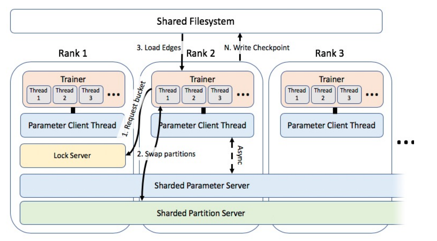
Here is the overview of the distributed training system, it requests similar types of communication. First we need to synchronize the bucket access and we need to exchange model predictions once you have done training a particular bucket. There is also some common shared parameters across different machines, those are the parameters of the relation types and is stored in a shared file system. Because of the number of shared parameters is relatively small compared to the giant embedding tables that we are learning, this scales almost linearly by the number of machines or trainers in the system. So if we train this on say 40 machines, you almost get 40x speed up for larger embedding tables as well. So overall this enables us to chain on giant embeddings efficiently.
Embeddings: Additional Topics
So far we learn about word and graph embeddings in euclidean distance. More recently, there is an interesting body of work on hierarchical embeddings, learning hierarchical representations representations by embedding entities into hyperbolic space using concrete distance. The key idea behind is with the natural geometry of the hyperbolic space, the embeddings learnt discovers hierarchies from similarity measurements, which often exists in data.
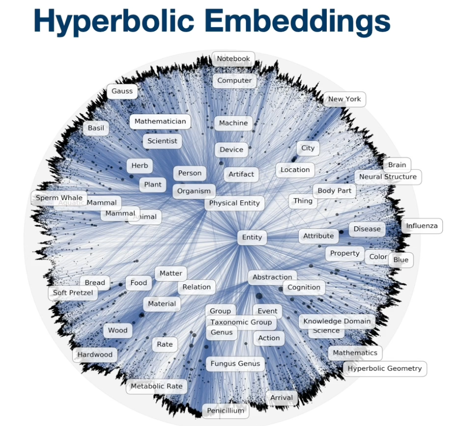
For instance, if you see the graph on top, you can see that vector of more general category entities, such as the name entity is very close to the center of the space. Whereas a more specific term like sperm whale is far apart from center. So additional benefits of the hyperbolic embeddings is that it usually requires followers dimensions to represent those entities. For instance, dimension people usually use for word2vec is about 300 while in hyperbolic space, usually a dimension of ten is good enough to good quality embeddings. You can also infer hierarchical relationships from the embeddings.
Bias in word embeddings
Machine learning systems are found to be systematically biased, not only the bias come from the data set people use to train ml models, but it is usually the case that the bias is further amplified by the machine in a system, which can cause a lot of issues. As we rely on ML systems heavily these days, it is very important to make sure that our ML model did not exhibit or amplify existing discriminatory or unfair behaviors. In the case of word embeddings, it is known that training embedding such as word2vec, exhibits those kind of biases to some extent. Researchers have showed in the word embedding space, the relation reveals that men is to computer programmer as woman is to homemaker. It also showed extreme she occupations vs he occupation.
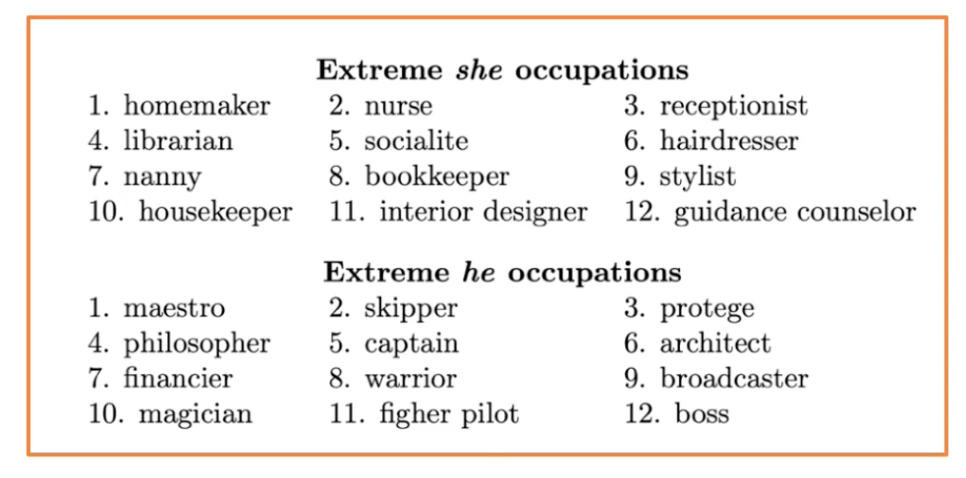
As we see in the list above, the node model exhibits existing biases towards occupations for different genders.
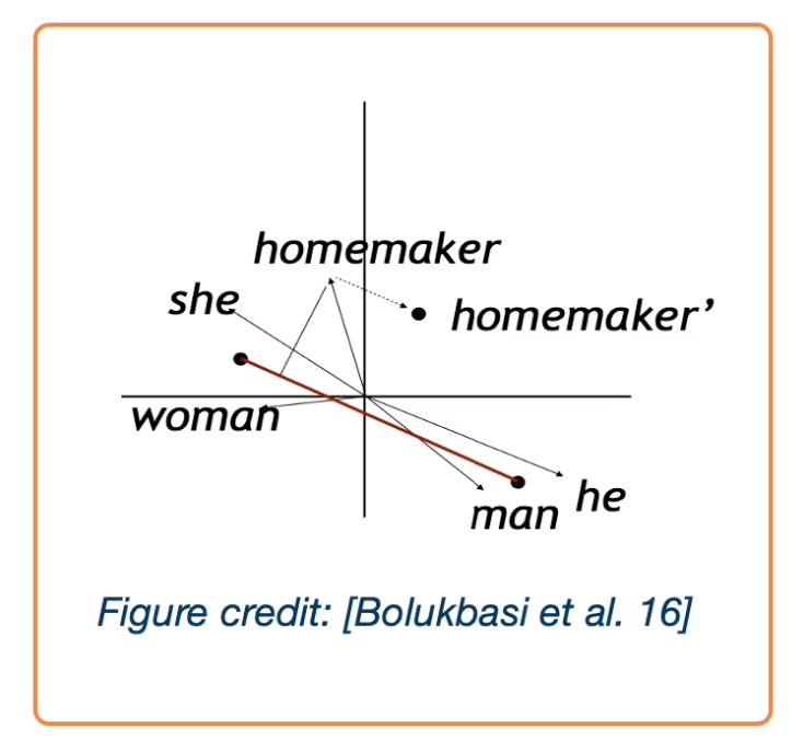
In their work, they also discuss how to debias and it is not an easy task. Here is an overview.
- identify gender subspace with gender words.
- Project words onto this subspace.
- Subtract those projections from the original word.
However…
- Not that effective, and the male and female words are still clustered together
- Bias pervades the word embedding space and is not just a local property of a few words.
Lesson 14: Neural Attention Models
Readings
Softmax and Preview of Attention
We are going to a review of softmax function, because we are going to use the softmax function as a mechanism for neural attention.
- Attention: Weighting or probability distribution over inputs that depends on computational state and inputs
- Attention allows information to propagate directly between “distant” computational nodes while making minimal structural assumptions.
- The most standard form of attention in current neural networks is implemented with softmax.
Softmax:
- For any inputs the softmax returns a probability distribution.
- Softmax is permutation equivalent (a permutation of the input leads to the same permutation of the output)
Recall that for softmax, the most mass of probability distribution lies on the largest input. So the softmax should be ArgSoftmax, so because it gives you a distribution, it is selecting from the inputs:
- Softmax interpolates between a distribution that selects an index uniformly at random
- And a distribution that selects the argmax index with probability 1
- softmax is differentiable
We can make this a little bit more relevant to attention by taking about vectors by making these vectors instead of real numbers, what we want to do is select vectors by how similar they are to a query:
- Given a set of vectors $\{u_1,…,u_N\}$ and a “query” vector $q$,
- We can select the most similar vector to $q$ via $p = Softmax(Uq)$
- We cannot use argmax because it is not differentiable
- $U$ is the vectors arranged as rows in a matrix
- This is the “softmax attention”
When softmax is applied at the final layer of a MLP:
- $q$ is the last hidden state, $\{u_1,…,u_N\}$ is the embeddings of the class labels
- Samples from the distribution corresponding to labelings (outputs) In softmax attention:
- $q$ is an internal hidden state, $\{u_1,…,u_N\}$ is the embeddings of an “input” (e.g previous layer)
- The distribution correspond to a summary of $\{u_1,…,u_N\}$
Attention
More generally, attention in the context of a neural network is a distribution over the inputs of that layer that depends on the computational state of the layer and the inputs themselves. We can talk about hard attention, which means you select one of the inputs or you select some of the inputs explicitly. Or soft attention where you compute some summary over the inputs.
The most common form of neural attention nowadays is softmax potential. In computer vision, a natural way of using attention is saccades, or deciding where to look based on what you have seen before and what is in the image currently. In these works, attention is over the set of spatial locations in an image - given current state/history of glimpses, where and at what scale should we look next?
Attention also ahs a pretty long history in NLP, in particular in translation there is a notion of alignment.
Native alignment is if you are translating a sentence from one language to another. In the picture there we are translating german to english. If you are translating a sentence from oen language to another, you might expect that there is some loose correspondence between the words in the sentences. So it doesn’t necessarily need to be exactly one to one, its just for each english word in the target sentence, maybe there is some german word in the source sentence that maps to it. And the order isn’t going to be preserved and it doesn’t, again, even need to be an exact correspondence. Maybe one word in English corresponds to a set of words in German. And so a soft alignment is a way of making this notion precise. It is for each word in the target, you have a distribution over words in the source, it is for each word in the target, you have a distribution over words in the source. If you think about it, that is attention just as we have talked about it before. The computational state is where you are in the sequence as you are translating and the input is the source sentence. So you have a distribution over the input, which is the source sentence, that depends on the computation state which is where you are in the translation, and the input itself.
Attention as a neural network layer explicitly seems to be pretty surprisingly new and it only became popular, very, very recently, and part of that is just due to the hardware we had and the training techniques we had. Making things train successfully with neural attention is a little bit more tricky than training conv nets or fully connected networks.
Current (Standard) Approach to (Soft) Attention
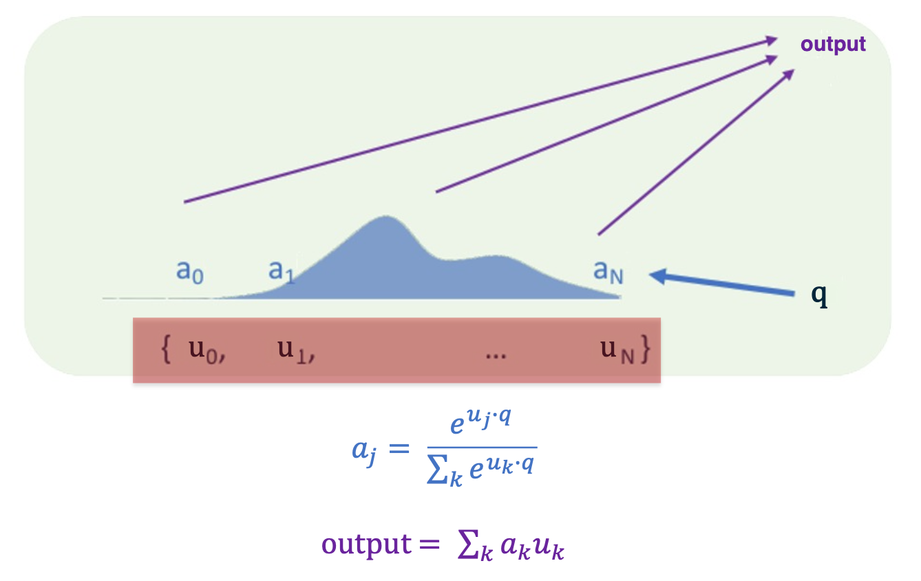
The way it works is you input to the layer a set of vectors which are highlighted here in red, the $U$. We are going to take this set of vectors and inner product each one of these vectors with a controller $q$. The controller is part of the layer’s state. We will talk about where that might come from in a little bit. you take that controller state and you inner product against each of the $U$, which again is a set of vectors, not a sequence of a list or anything ordered.
So when you inner product the controller state against $U$, you then take the softmax of that set of numbers and that gives you weights a:
\[a_j = \frac{e^{u_j \cdot q}}{\sum_k e^{u_k \cdot q}}\]So now we have this set of weights, that have been obtained by softmax of the controller against the inputs, and the output for the module is summing up the inputs with the weights given by the softmax function that we computed previously. This is soft attention in its simplest form. There are other more complicated things you could do, for example you could have the inputs $U$ be stacked as $Us$ and $V_s$ where the $Us$ are called the keys. The keys would be used to compute the softmax weight and the $Vs$, the values, would be used to compute the output. There are other transformation you can apply other than just summing the things up.
An important property of softmax attention as a layer, or attention as a layer more generally, is that the representational power grows with the size of the input. So in contrast to, for example, a fully connected layer, which can just take an input of a fixed size or a classical recurrent network, in which case the representational size is the same, independent of the length of the sequence that you feed into it. A softmax has a hidden state that grows with the input and and that is one of the secrets of its power.
Multi-Layer Soft Attention
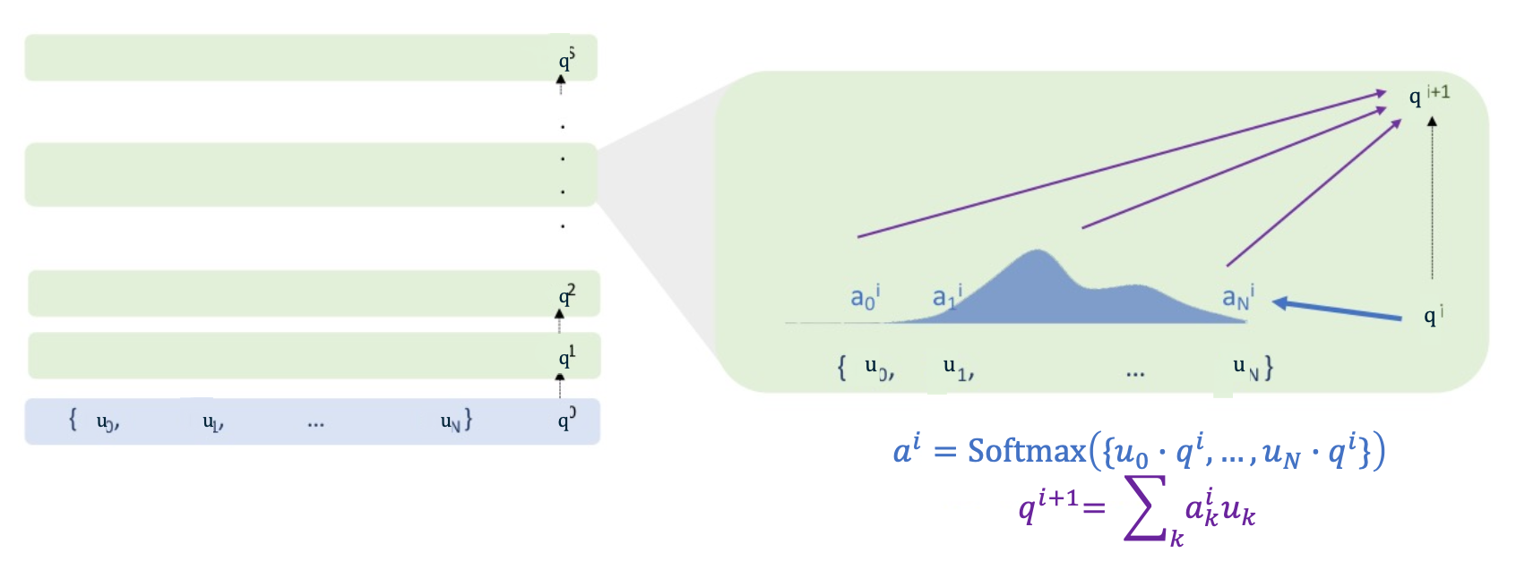
Here we are showing one example of a multi-layer neural attention model. And in this model, the hidden state of the model is the controller, q. And so the controller at $q^0$, the initial controller state, comes from somewhere (we can talk about where that might come from or it might be set all to 0). Then the inputs to the network are the same as in the previous parts where the inputs to the layer were a set of vectors. So we have the inputs to the network being a set of vectors and some initial controller state $q^0$. And we update $p^1$ via the softmax attention exactly as we saw before, and that is described on the right. And after one layer of softmax attention we get a new controller state $q^1$. The new controller state is used to compute the next softmax attention layer with the inputs being the $U$ as before, and keep repeating that over and over again. So each layer of the network is softmax attention and the hidden state is the controller.
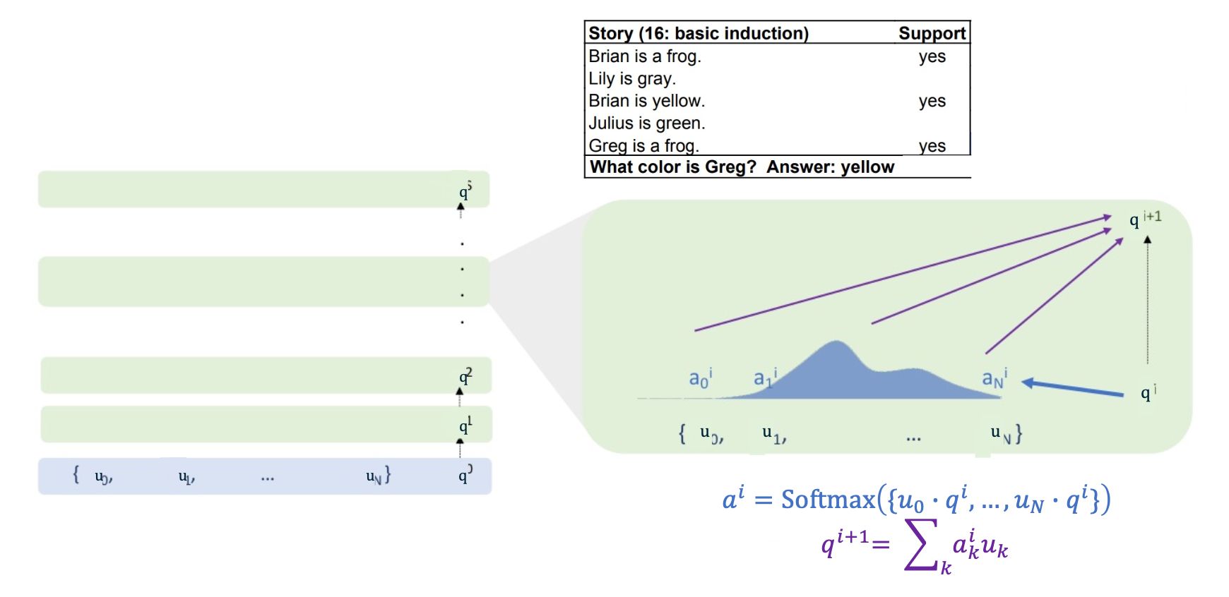
Watch this in action for an example, so the example comes from baby tasks, and what we have is a little story to guess. So the story is Brian’s a frog, Lily is gray, … , Greg is a frog. And then the model is expected to answer a question about the story. So here the question is what color is Greg?
And the idea is that well, the model should recongnize that Brian’s a frog and Brian is yellow. So if Greg is a frog, Greg should maybe also be yellow. (You may not buy the logic of the problem but thats how the model is being trained to do that kind of induction)
The inputs to the network, the $U$, are going to be the encodings of each sentence in the story. So for example $u_0$ is some encoding of Brian is a frog, $u_1$ is encoding of Lily is gray and so on. The initial controller state is going to be an encoding of the query “What color is Greg?” using similar sort of encoding to the previous sentences.
Now once we have done this encoding, then $q^0$, which ahs the encoding of what color is greg in it, has the largest inner product with “Greg is a frog” amongst all the sentences in the story because it has the word Greg in it, and “Greg is a frog” has the word Greg in it, and none of the other sentences have any word overlap or any kind of other overlap with what color is Greg. Thus, $u_4$ gets the bulk of the attention weights. So $a^4$ has the largest attention weight. And then when we compute the updated controller state as a weighted sum of the encoded sentences, the updated controller state is mostly the encoding of Greg is a frog. Then, we take that updated controller state, and, again, inner product it against all the inputs. (We do not directly use the weighted sum, we make a rotation of a transformation projection of it so that you do not want Greg is a frog to have the biggest inner product with Greg is a frog, so the rotation is there to stop it from happening). After that, the encoding Greg is a frog which is what is sitting in the controller state or $q^1$, has highest inner product with Brian is a frog. The same story unfolds and most of the attention weight is going to be on Brian is a frog, and when you make a weighted sum of all the sentences encodings with that weight, then as you update the controller state $q^2$, the controller state is basically going to have Brian is a frog. (Similar rotation is applied so you do not attend to the memories you have attended to before)
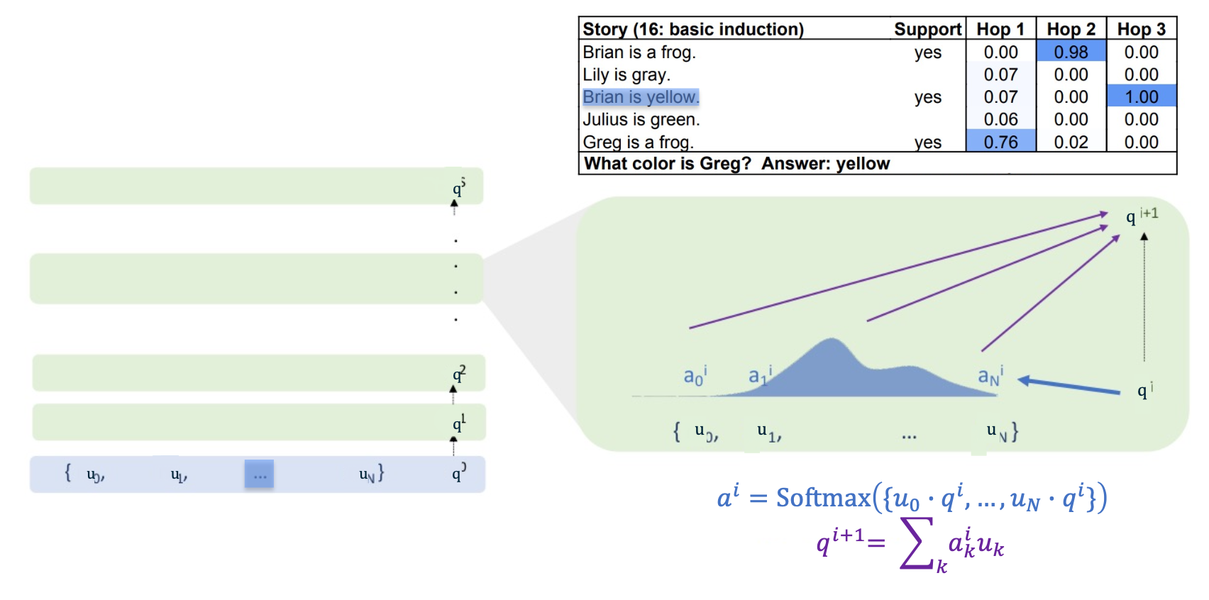
Continuing in the same way, the controller state now has the encoding of Brian is a frog in it and has been rotated so you cannot hit inputs that you have hit before, so the maximum inner product is on Brian is yellow, because you have the Brian and the Brian. So when we repeat the same update to the controller state, we end up with Brian is yellow in the controller state. Finally, we want to output something and so the machine knows enough what a color is and can match the color to the yellow that is in the controller state. And so the final output layer when it looks at the controller state can pick out the yellow and answer yellow. And this is how this kind of multi-layer attention can do reasoning over a set of inputs, reasoning over a set of quotes.
So everything we have talked about has kind of taken the input set as a set, as a pure set, and a lot of times that is not ideal. Even in these baby stories just discussed, it can be useful to know the order of sentences if there is some temporal information there. More generally:
If inputs have an underlying geometry, can include geometric information in the weighted “bags”. The most standard piece of geometric information you have is sequence order, if the inputs have a temporal structure or casual structure, you can use that. The most standard way people use that is with position embedding. Position embedding is simply a vector that depends only on the location in the sequence which is added to an input that is placed at that location in the sequence.
Example: For sequential data, use position encoding, given the “location” in the sequence of that inputs.
- For each input $m_j$ add it to vector $l(j)$
- $l(j)$ can be fixed during training or learned
- For example, a sinusoid of varying frequency in each coordinate
Transformers
Transformers are a multi-layer neural attention model that is currently state of the art in most language tasks and beyond their state of art in some audio tasks even, and some vision tasks. Has superior performance compared to previous attention-based architectures via
- Multi-query hidden state propagation (or known as self-attention)
- Multi-head attention
- A bunch of things that improved the performance such as Residual connections, LayerNorm, other things that stabilize the training of neural networks.
- These benefit most networks and not just transformers.
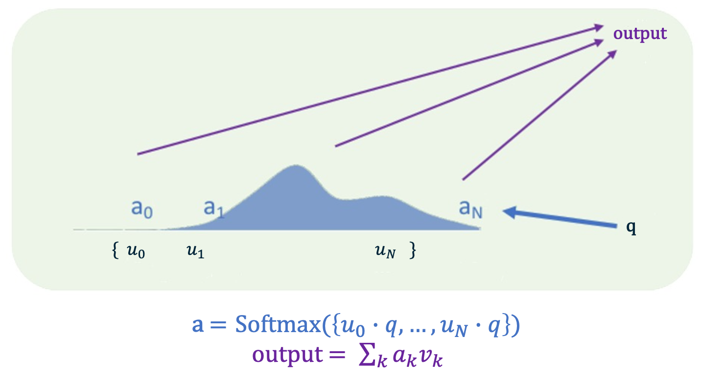
Recall that we can do more complicated things, such as using $u$ to calculate the softmax weights, and Values $v$ are used to compute the output.
Self-attention
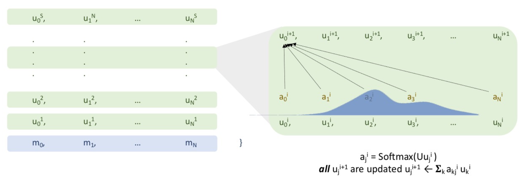
In the previous section, we showed how a multi layer softmax attention network works. Self attention like in a Transformer improves on this by having a controller state for every input. And in the same way, attention has an advantage over say recurrent neural networks, and that the hidden state grows with the size of the input. A transformer or other self attention style network has an advantage over the previously shown simpler multi layer attention network and there is a controller for every input, so the size of the controller state grows with the size of the inputs.
The way it works is each input has a controller state living over it, those are the $u^j$ and those controller states, each one of them are updated with softmax attention just as the multi layer attention network shown previously did.
Multi-head attention
Multi head attention splits up the controller states into chunks and operates the self attention on each chunk separately and then recombines with a fully connected network.
- Multi-head attention combines multiple attention “heads” being trained in the same way on the same data - but with different weight matrices, yielding different values
- Each of the L attention head yields values for each token - these values are then multiplied by trained parameters and added.
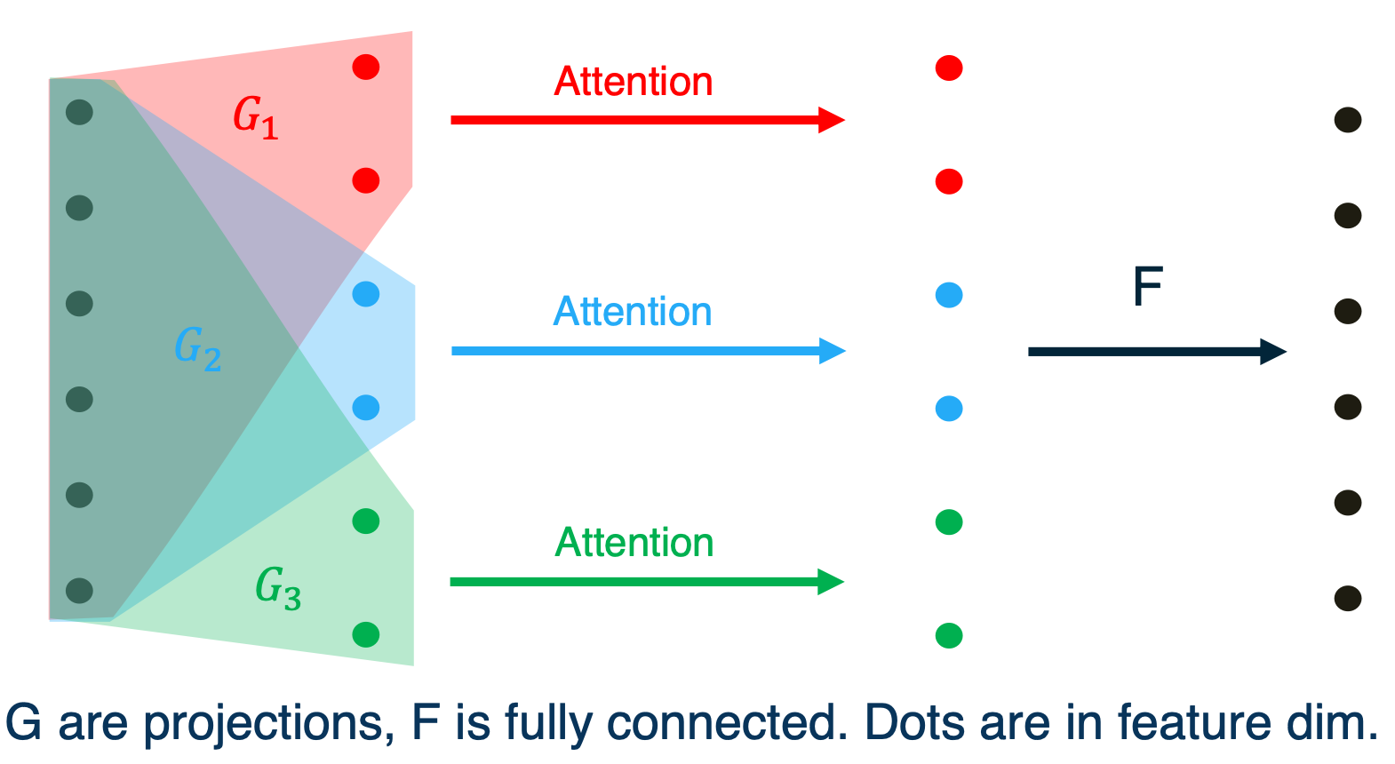
So it looks like this, on the left, we see the input controller state. We take some projections which we will call G and take the full state and map it down to smaller sub states. On each of the sub states, we run attention, we get attention weights for each of them, and then sum up as normal. So we do our weighted sums with the attention that was computed on each chunk and then we take a fully connected network, that is the mapping from the colored dots to the black dots. We take a fully connected network to combine all of the chunks.
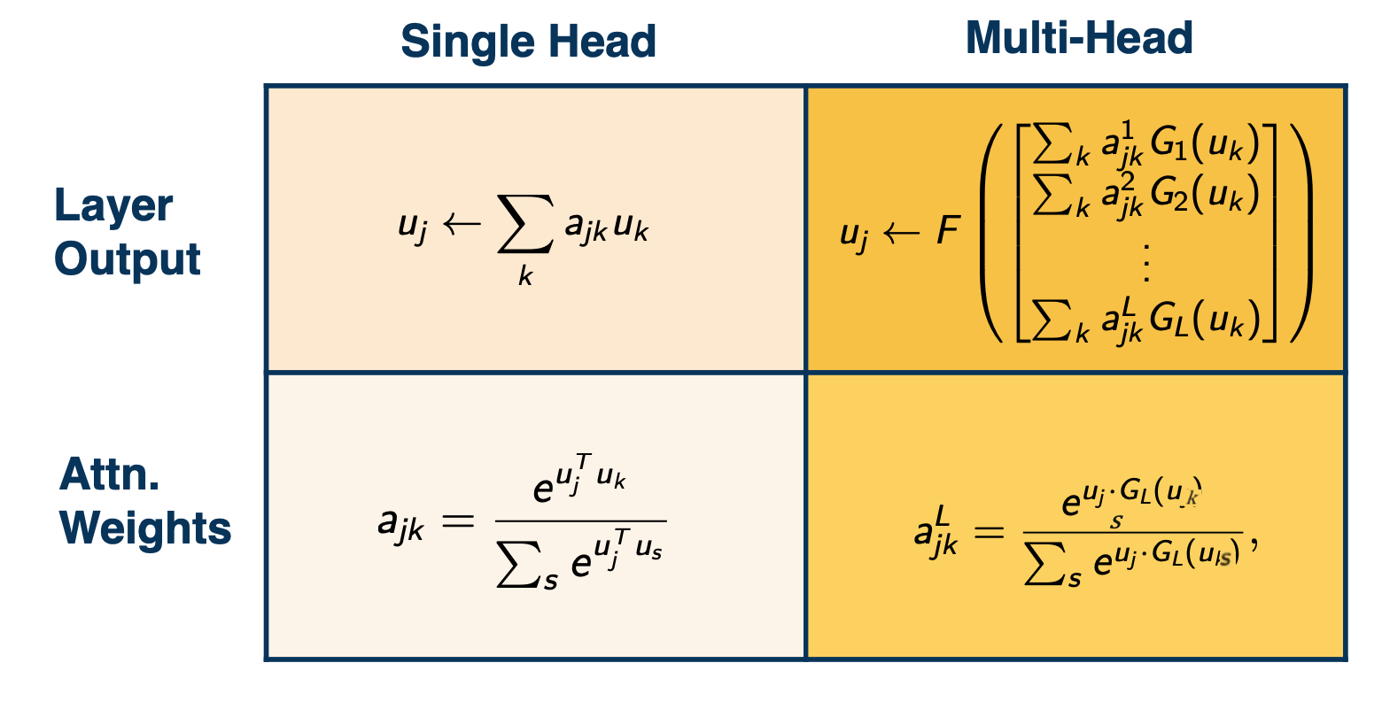
In equations this looks like this, where as for the attention weights of the single head attention that is the bottom left corner. We take the inner product of each input with its controller state and take the softmax of that. In multi-head attention we first project the controller state to L different chunks and we compute L different sets of weights. And for the recombination in the top left, we see single head attention, we just sum up the weights against those inputs. In multi head attention (on the top right) we first sum up each head independently. And then we apply a fully connected network to recombine.
Residual connections, LayerNorm
Nothing much other than how these has helped all kinds of neural networks, and not just transformers.
As a last point, While Transformers operate on sets of vectors (or graphs), because you can mask out certain locations of the attention based on a graph structure. However in this notes, they were introduced in the setting of text so they became famous in the context of state and are really state of the art as NLP models.
There is a bunch of things that people tend to do specifically for NLP:
- Position encodings depending on the location of a token in the text
- For language models: “causal attention”
- e.g in language, we mask out attention weights that do not go from left to right. (since you only read text from left to right)
- Training code outputs a prediction at each token simultaneously (and takes a gradient at teach token simultaneously)
- By not inputting a sequence and outtpuing a single output to be checked, but rather over each input token, you output token at the same time.
- For example for language model, instead of reading the context and outputting the next word, at every word in the context, you output the next word simultaneously. This multiplies the speed of your training by the size of the context. In order to do that, for language modeling, you have to use the casual attention described above.
- For math language models like BERT, you do not need casual attention and you can make an output at every token simultaneously without using casual attention.
Lesson 15: Neural Machine Translation
Readings
None!
Neural Machine Translation
Translation is hard problem
There are many correct translations for a typical input sentence.
Language is ambiguous
- The professor said on Monday we would have an exam
Language depends on context
- I saw her duck 🙇
- I saw 👁 her duck 🦆
- I saw
 her duck 🦆
Languages are very different in structure which can sort of make it particularly different to go from one to another.
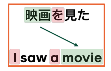
Here we see an example of simple sentence both Japanese and English where we can see the object word for movie are in very different parts of the sentence. And each language uses particular types of function, which might not be explicitly used like the object marker in japanese and the pronoun and article in English.
Machine Translation
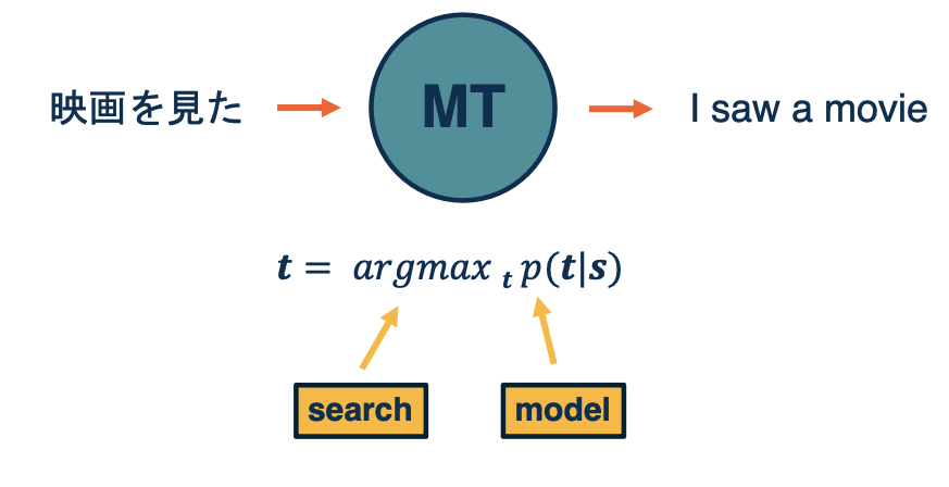
Let’s take a look at how Machine translation approaches the problem of translating automatically. So the general structures, is you want a sentence in one language t o come in, e.g In Japanese and want to output English. The way we are going to break this down as a machine learning problem is, will represent the probability of the target sentence, the English sentence here. Given the four particular source sentence, since the sentences the output is composed of a sequence of tokens, probably each word, I saw a movie the decision is not as simple as a simple classification. so we are going to need some way of doing search over the exponential space of possible output tokens, that is what is represented by this argmax here. We want to approximate the best target sentence for a given input.
Sequence Generation is Autoregressive
Translation is often modeled as a conditional language model where you have a language model over target tokens and is conditioned on the source sentence.
\[p(t\lvert s) = p(t_1\lvert s) \times p(t_2\lvert t_1,s) \times ... \times p(t_n \lvert t_1, ..., t_{n-1}, s)\]Probability of each output token estimated separately (left to right) based on:
- Entire input sentence (encoder outputs)
- All previously predicted tokens (decoder “state”)
- Language has a left to right property, we will see in a ML model leads to what we call auto-regressive generation.
The other problem is exact search $argmax p(t\lvert s)$ is intractable
- Exponential search space of possible sequences
- Estimated by beam search (covered shortly)
- Typical beam sizes: 4 to 6
Seq-to-Seq Models
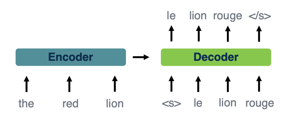
This image models the sort of overall structure,that sort of overall framework and two, which will fit our neural network models to do what we call sequence to sequence learning. Where in some way we will get an intermediate representation of the entire source sentence, and what will be called the encoder. And then the decoder will be using that input predict output tokens one at a time. So you will have some notion of that each step is putting the previously predicted token in addition to considering the encoder, which you see here. And these tokens will be represented by word embeddings which you have seen before.
Beam search
So the way we are going to approximate the argmax, so the most likely target sentence is using beam search. Very simply, that means we are going to explore a limited number of hypothesis at a time, that number will be called the beam size $k$. So here, we see a simple model where the beam size is two. So at each step, we are considering two possible total sequences. And the first step we have the two most likely top words, the D, and dog. Now, we are going to expand each of those into most likely tokens, so here, we are seeing in the next step, we have the top four most likely sequences expanded just by taking hte top two of each, and then we will take the top two overall to expanded it in the next step.
In a nutshell:
- Search exponential space in linear time
- Beam size $k$ determines “width” of search
- At each step, extend each $k$ elements by one token
- Top $k$ overall then becomes the hypothesis for next step
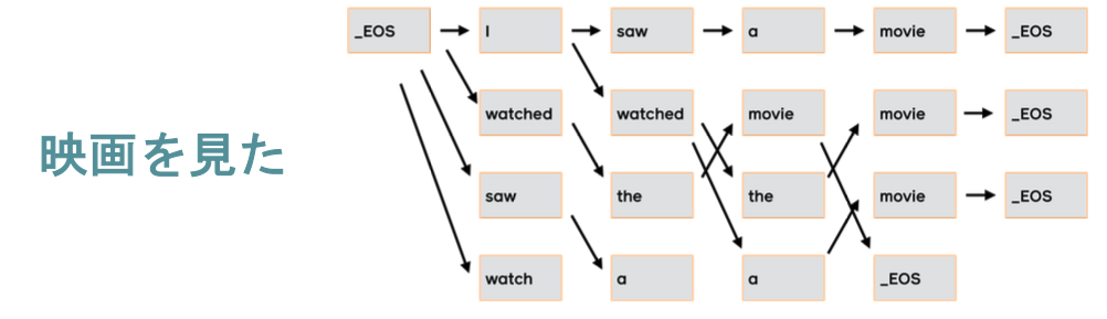
To make it more concrete, this is what beam search might look like for a full translation example, again translating that same JApanese sentence into English. So you can see that based on the overall probabilities at each step, the different hypothesis can be expanded into the next step.
Neural Machine Translation Architectures
Finally, this is an overview of the sort of specific types of neural networks you might see plugged into that encoder decoder spot.
- RNN (typically LSTM) (When neural machine translation gained traction, these were typically recurrent neural network models, which makes sense when you consider language is fundamentally a sequence)
- Bi-directional encoder
- Since you know the entire sentence at once, and then a unidirectional left to right decoder.
- Major breakthrough: encoder-decoder attention
- Bi-directional encoder
- Convolutional
- Encoder and decoder based on fixed-width convolutions
- Here we would be dealing with a 1D convolution over the sequence length.
- Simple activation function (Gated linear units)
- Encoder and decoder based on fixed-width convolutions
- Transformers
- Architecture used in most recent work
- Originally proposed for machine translation
- full self attention on the encoder and casual self attention on the decoder.
- Though now especially well known due to BERT and friends
Inference Efficiency
Inference Efficiency is an important topic because these sequence to sequence models for state of the art translation can be very large in particular while training it can be expensive.
Whats expensive?:
- Step by step computation (Auto-regressive inference)
- Output prediction: Θ($\lvert$ vocab $\lvert$ * output length * beam size)
- Deeper models
Strategies:
- Smaller vocabularies
- More efficient computation
- Reduce depth/increase parallelism
Vocabulary Reduction
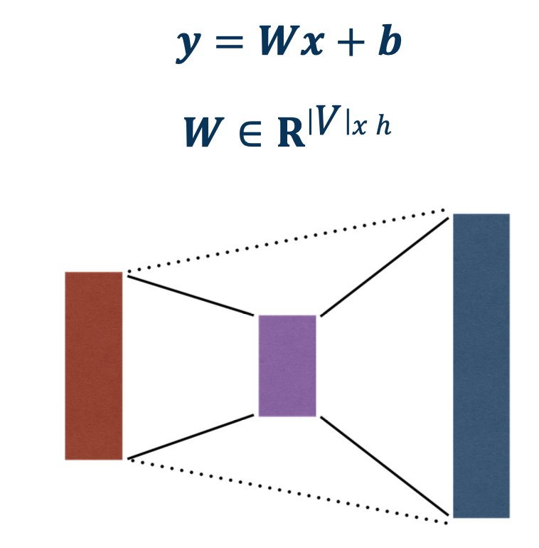
- Large vocabulary makes output projection expensive
- Can address this by subsetting the vocab, e.g taking out uncommon words.
- However not all tokens likely for every input sequence
- IBM alignment models use statistical techniques to model the probability of one word being translated into another
- Lexical probabilities can be used to predict most likely output tokens for a given input
- Achieved up to 60% speedup
Byte-pair encoding
- Languages have very large (or open-ended) vocabularies
- Problem: how to model rare or unseen words
- Character models are general but can be too slow in practice
- Subword models solve this by breaking up words based on frequency
- One widely used algorithm is byte- pair encoding (BPE), illustrated at right
Example of byte-pair encoding:
- Byte-pair encoding comes from compression, where the most frequent adjacent pair is iteratively replaced
-
Example consider this string
abcdeababce -
Step 1 replace most frequent pair “ab” by “X” (and add replacement rule),
XcdeXXce -
Step2 replace next most frequent pair (e.g Y=Xc) yielding
YdeXYe, soX=abandY=Xc
Layer Drop
So you can think of this analogous in some way to drop out, at least for training. You are not going to use every layer for training so you drop them with some probability and then at the end to get a faster network for inference time, you can select layers to prune. This gives you a smaller model with a good trade off with only slight decrease in performance and accuracy, but much faster because you are not doing every decoder layer.
Hardware Considerations
Inference is faster on specialized hardware (GPUs, TPUs, etc.)
Batched vs. on-demand: average efficiency can be increased by translating multiple inputs at once
- Especially with accelerators (GPUs, TPUs, etc.)
- However may not be practical for real-time systems
Big speedup from parallel computation
- Especially with accelerators
- Autoregressive inference time dominated by decoder
Quantization
- Computation time is dominated by matrix multiplication
- Inference can be sped up by performing operation in lower precision domain
- Training quantization also possible (e.g, FP16 on current Nvidia GPUs)
Non-autoregressive Machine Translation
One of the big sort of bottlenecks that slows down computation is the need to predict each token in the output sentence one after another. So the idea here is to get around this by predicting all of the tokens at once. So that is challenging and not quite state of the art yet. The reason for that is because you have to figure out some way of coordinating all the sequences. You are doing structured prediction, right? Each token has to work together rather than be predicted in isolation. But there has been a lot of varied work on this recently and it is exciting new direction for future research and sequence generation.
Lesson 16: Advanced Topics: Translation at Facebook and Automated Speech Recognition (ASR)
Readings
- CTC based ASR Systems: Connectionist Temporal Classification: Labelling Unsegmented Sequence Data with Recurrent Neural Networks (Links to an external site.)
- RNN-T based ASR System: Sequence Transduction with Recurrent Neural Networks (Links to an external site.)
- RNN-T Contextualization with Biasing and Attention Module: Contextual RNN-T For Open Domain ASR (Links to an external site.) <!– <iframe class=”embed-video” loading=”lazy” src=”https://www.youtube.com/embed/10oQMHadGos” title=”YouTube video player” frameborder=”0” allow=”accelerometer; autoplay; clipboard-write; encrypted-media; gyroscope; picture-in-picture” allowfullscreen
</iframe> –>
Translation at Facebook
- Have a language identification module that runs for every single piece of text that is produced by Facebook and it assigns it.
- Language score - the most likely language that this piece of text is in.
- Have a user language model that tells us what are the likely language a certain user understands.
- Based on the history on how much they communicate in a certain language or how much they consume content in a certain language.
The tricky part when we detect that a certain user cannot understand the content because it is in a different language, we provide the option to see translation. There is a little button where if the user clicks it, the user is accessing the translation in their language of preference.
Translation Challenges: Low Resource
Challenge 1: Social media text can be short, error phone, new words, hashtags etc. Emerging languages are also a challenge, this brings about a lack in data.
NMT (Neural Machine Translations) systems have a steeper learning curve with respect to the amount of training data , resulting in worse quality in low-resource settings, but better performance in high- resource settings. For example if you to go rarely used languages, you barely have 10,000 sentences to train on.
Challenge 2: Language similarity
Languages that tend to be linguistically very close to each other say English and Spanish or English and French. And in reality, many of the languages that we need to learn to translate are not very well related to English.
Challenge 3: Domain
Even if we have some availability of data, it is quite possible that it is not in the right domain, is not geared towards our needs. So for example if you want to learn to translate news, you may have available data that is related to baboons to manuals or that is related to medical terms, but not necessarily in the area that you want to learn.
Challenge 4: Evaluation
For many of the language pairs that we will like to improve, we do not have access to a real test set. It is often emulated by ablating or reducing high resource language pairs which they do not correctly represent the reality of a low resource situation.
The team mainly worked on challenge 4, which gave birth to the Flores project.
- started with open source data, wanted to have a rich combination of different domains in test set; choose wikipedia nad sampled different domains coming from science, religion, business, sports, etc.
- Then, send these sample documents to translation. Due to low resource, automatic checks are required and then 2 Human translations is required to audit the translations.
- Then run human checks again, those with poor quality is sent back
- Finally collect the results which enables a high quality benchmark set together with some training data that we publish so researchers could actually start making process in solving the low resource language.
One of the most powerful techniques is Multilingual Training. It exploits the relatedness between certain languages, if one is resource poor and another one is resource rich, we can do some transfer learning. For example when you have languages like Ukrainian and Belarsian which belong to the same language family, lexical to semantic etc. Nowadays you have modern models like the G sharp which are actually embedding 100 languages into a single model to be able to translate to English.
Another technique that has been used quite extensively is back translation. This same supervised technique allows us to leverage large quantities of monolingual data, which we then use to train a larger model. This works very well for languages like German and English, and has helped to bring equality to a level that has won several translation competitions.
How does this work? You have some small amount of training data say from German to English, you train the small model, German to English, you then use to annotate large quantities of German data into fake English data, or translated English data. And now, you use this pair, you reverse the order and you use it in conjunction to your previous data. So now you can train a better English to German system. This has worked well for high resource languages but not so for low resource language. Because in the low resource condition, the intermediate model is so weak that the data that you generated is not good enough.
So here comes iterative back translation,
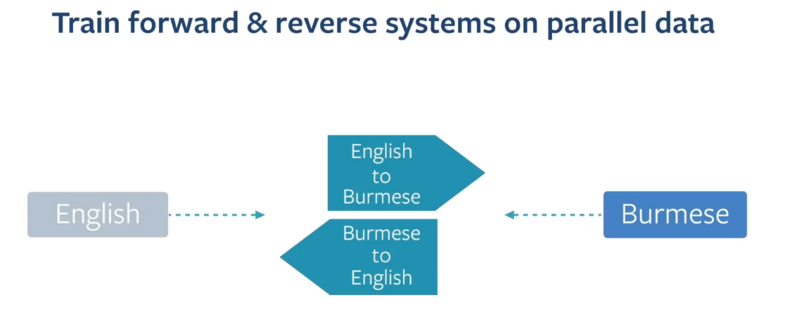
We take the same idea by constellation, but do it in several stages.
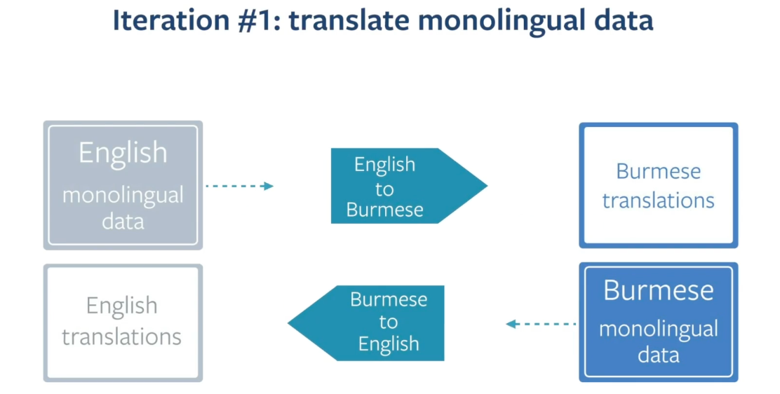
First, you train intermediate English to Burmese and vice versa, which you then use to translate large quantities of monolingual Burmese and English data.
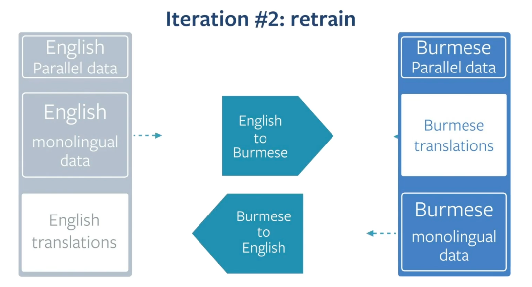
Then you repeat this operation, you take this, the data that was generated by these models and train at second iteration intermediate model that you then use to translate more monolingual Burmese and more monolingual english data and so on.
Another way to do this can be:
- Language Agnostic Sentence Representations
- Web scale mining
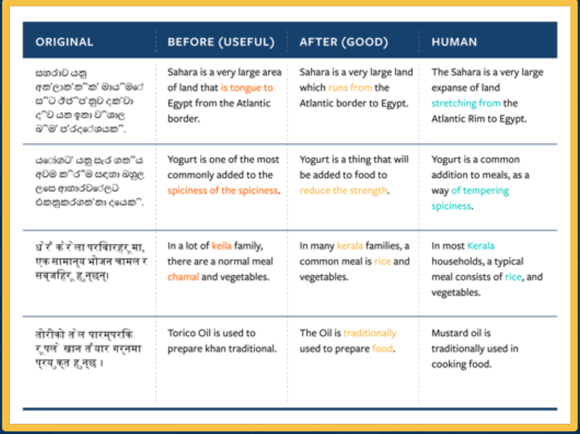
Rethinking Translation Quality
It is possible that translations goes horribly wrong. e.g when we translate “good morning” into “attack them” or names of public figures have been misunderstood, resulting in offense translations.
One idea is to use a quality scale:
The problem is this scale is not continuous, and sometimes a small mistake can led to a catastrophic translations. Those are the ones that would lead to a terrible experience for users.
So what are catastrophic translations? Here are some examples:
- Bad Named Entity translation (El Centro, CA -> The Center, CA)
- Wrong pronouns (it, he instead of she)
- False profanities ( Mr sh*thole)
- Implausible translations (a water treadmill)
- Introduction of violent terms (“attack them”)
One possible solution is to design the modeling and the measurement of translations quality centered around user experience.
- Catastrophic-aware translation systems
- Able to explain the type of mistakes they believe and what reasons they believe so
- Quality metrics that account for critical mistakes
- AI Systems with more transparency and control
Different Approaches for ASR: Readings and Additional Resources
Look at one type of ASR (Automatic Speech Recognition) which is the RNN-T. For the remainder of this lesson (16) RNN-T stands for recurrent neural network transducer based ASR systems.
These Sections are not covered as they are not related to the assignment + your time is better spend on reading the “attention is all you need paper”!
- Introduction to Different Approaches for ASR
- Task of Automatic Speech Recognition (ASR) System
- Modularized (Hybrid) ASR
- Non Modularized (End2End) ASR
- RNN-T Training
- RNN-T Decoding: How to Utilize RNN-T Model at Test Time
- RNN-T Greedy Decoding
- RNN-T Beam Search Decoding
- RNN-T Personalization
- Different Approaches to ASR Conclusion
Module 4: Advanced Topics
(At this stage I am a little tired of creating the notes by now, and it is no longer involved in any projects)
Lesson 17: Deep Reinforcement Learning
Readings
Reinforcement Learning Introduction
Reinforcement learning is the Sequential decision making in an environment with evaluative feedback.
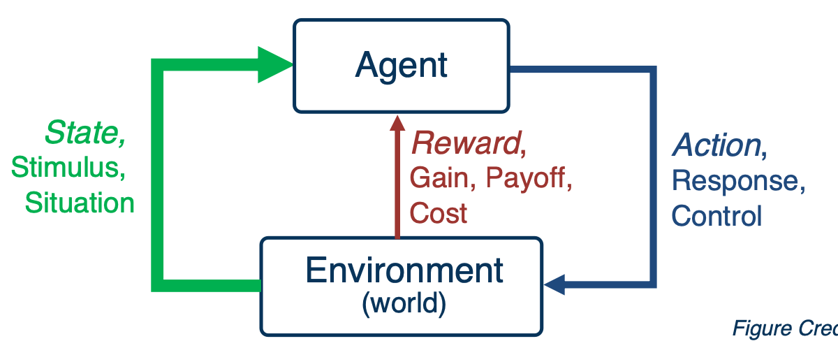
- Environment may be unknown, non-linear, stochastic and complex.
- Agent learns a policy to map states of the environments to actions.
- Seeking to maximize cumulative reward in the long run.
Evaluative Feedback
- Pick an action, receive a reward (positive or negative).
- No supervision for what the “correct” action is or would have been, unlike supervised learning
Sequential Decisions
- Plan and execute actions over a sequence of states.
- Reward may be delayed, requiring optimization of future rewards (long-term planning).
Signature Challenges in Reinforcement Learning:
- Evaluative feedback: Need trial and error to find the right action
- Delayed feedback: Actions may not lead to immediate reward
- Non-stationarity: Data distribution of visited states changes when the policy changes
- Fleeting nature of time and online data
For RL to work, it needs a environment interaction API. In other words:
- At each time step $t$, the agent:
- Receives observation $o_t$
- executes action $a_t$
- At each time step $t$, the environment:
- receives action $a_t$
- Emits observation $o_{t+1}$
- Emits scalar rewards $r_{t+1}$
Markov Decision Processes
- MDPs: Theoretical framework underlying RL
- An MDP is defined as a tuple $(S,A,R,T,\gamma)$
- S - set of all possible states
- A - set of possible actions
- $R(s,a,s’)$ - distribution of reward
- $T(s,a,s’)$ - Transition probability distribution
- $\gamma$ - Discount factor
- Interaction trajectory: $… s_t, a_t, r_{t+1}, s_{t+1}, a_{t+1}, r_{t+2}, s_{t+2}, …$
- Markov property: Current state completely characterizes state of environment
- Assumption: Most recent observation is a sufficient statistics of history
In Reinforcement learning, we assuming MDP with unknown transition probability distribution T, and reward distribution R.
Evaluating feedback comes into play, and trial and error necessary.
For this lesson, assume that we know the true reward and transition distribution and look at algorithms for solving MDPs i.e. finding the best policy
- Rewards known everywhere, no evaluative feedback
- Know how the world works i.e. all transitions
A Grid World MDP
Let’s take a look at a simple environment
The 2D environment above is a grid world, where there is an agent indicated by a blue triangle, where the state of the environment is the agent right now is at $(2,3)$. The actions that the agent can take is either move one cell north, east, south, or west. The rewards are either +1 or -1 at the absorbing states shown in the figure above.
With this setup, it is easy to see that the optimal policy is to head east twice in order to reach the +1 absorbing state. However, let’s assume that there is some noise in how the agent transitions to next state. This noise is in the form of a 20% chance, of the agent drifting once a left or right of the direction of motion.
Now, things get a bit complicated the policy will now have to prescribe an action, for the states that the agent could land up in as it is not guaranteed to always move in the direction of east. One way to describe such a policy would be in the form of a 2D matrix of the same shape as this 2D grid, with each matrix element is prescribing an action to take if the agent is at that cell. This leads us to the formal definition of a policy, that we will use for solving MDP.
Solving MDPs: Optimal Policy
Formally, a policy is a mapping from states to actions in which a single action is prescribed at each state.
- Deterministic - $\pi(s) = a$
- This is defined by a $n \times 1$ tensor.
- Because there is only 1 action possible at each state.
- This is defined by a $n \times 1$ tensor.
- Stochastic $\pi(a \lvert s = P(A_t = a \lvert S_t = s))$
- This is defined by a $n \times m$ tensor.
- finite set of n states and finite set of m actions
- This is defined by a $n \times m$ tensor.
so, what makes a good policy?
- Maximize current rewards? Sum of all rewards?
- Discounted sum of future rewards?
For this lecture we are going to use the discounted method, which is the factor $\gamma$.
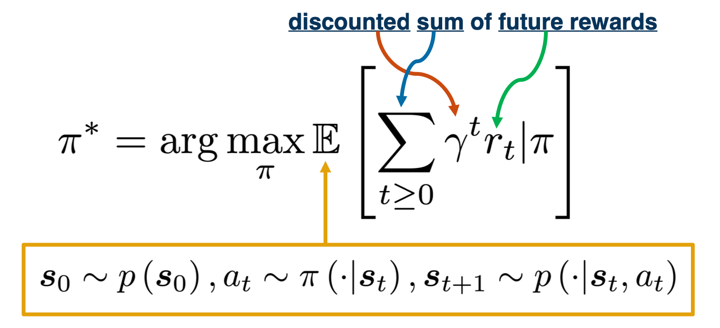
There are three random variables involved, the distribution over initialization states, $s_0$, actions across policy $a_t$ and the transition distributions over next states $s_{t+1}$
Sum of discounted rewards prefers rewards now to rewards later (with preference increasing with smaller $\gamma$ ), where $\gamma \in [0,1]$
Let’s now look at how the optimal policy is sensitive to changes in the MDP. The three figures shown here are for the same 2D grid world environment with stochastic transitions as earlier but with a small modification. There is now a constant reward value at all non absorbing states, and this constant is set to three different values, corresponding to the three different figures shown here.
We can see that as this constant rewards decreases to $-0.4$, going from the left to the middle figure, the optimal policy starting from the bottom right of the grid, stops taking the longer route to get to the +1 absorbing state and instead a risker shorter path. Further, decreasing this constant to -2 in the right most figure, shows the agent directly jumps to -1 instead to incur a lesser cost.
Discounting Future Rewards
For example consider this, what would you do if $\gamma = 1$ or $\gamma = 0.1$?
Clearly if the discount factor is low, you would go and get the reward of 10 before going to 1. if the discount factor is high, you will just get the 1 immediately.
Value Function
Now that we have looked at how to map state to actions with the policy, let’s introduce a new quantity that will help measure the performance of a policy, at various states.
A value function can be intuitively thought of as a prediction of discounted sum of future rewards. First, we will introduce a state value function or V function as a mapping from states to real values. $V : S \rightarrow R$
That will provide information about how good a state is, in terms of future rewards. Similarly, a state action function or a Q-function, $Q :S \times A \rightarrow R$, which will inform us of how good is taking a particular action at a state.
Formally, the value function $V$ of a policy $\pi$ at state $s$ is defined as the expected sum of the discounted awards.
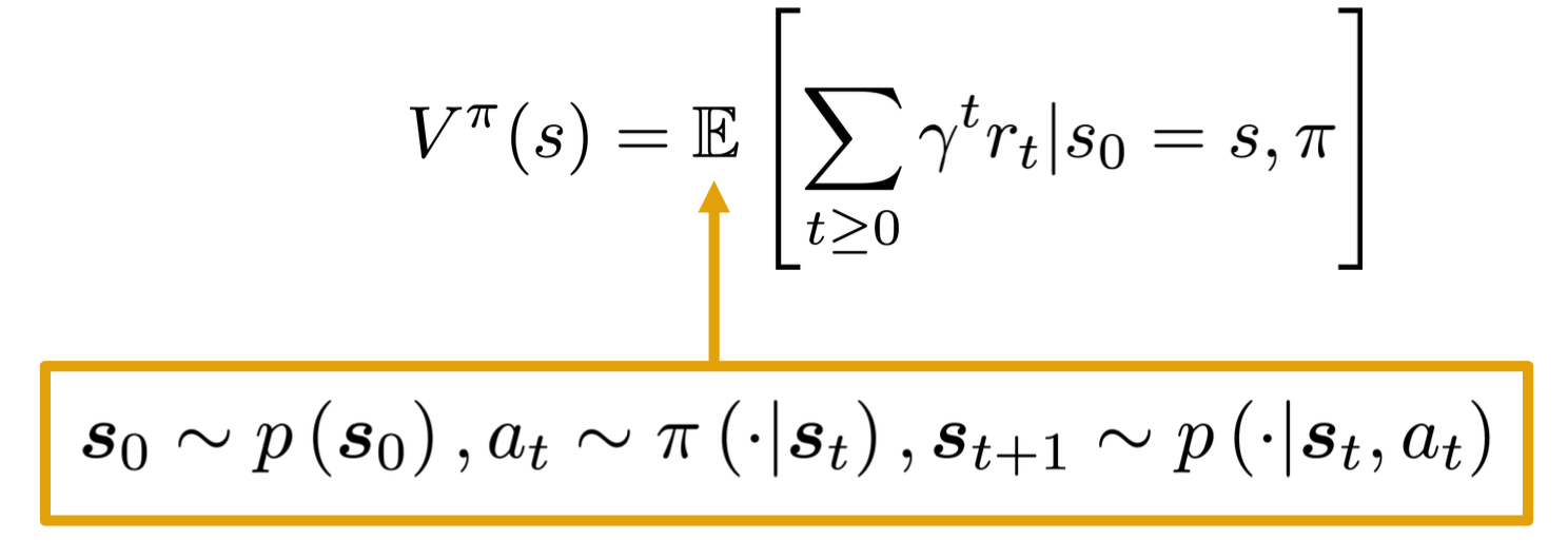
Similarly, The Q-function of the policy at state s and action a, is the expected cumulative reward upon taking action a in state s (and following policy thereafter):
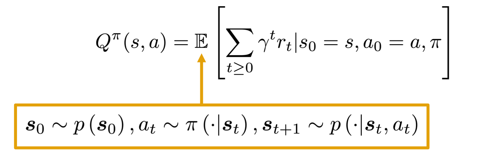
Algorithms for Solving MDPs
Recall in the previous lecture, we define $P_\pi$ and $Q_\pi$ for a particular policy $\pi$. Now we can also define the V and Q functions corresponding to the special policy or the optimal $\pi^*$ as $V^*$ and $Q^*$, in which cases we have just replaced the $\pi$ with $\pi^*$ in the definitions
\[\begin{aligned} V^*(s) &= \mathbf{E}\bigg[ \sum_{t \geq 0 } \gamma^t r_t \lvert s_0 = s , \pi^* \bigg] \\ Q^*(s,a) &= \mathbf{E}\bigg[ \sum_{t \geq 0 } \gamma^t r_t \lvert s_0 = s, a_0 = a , \pi^* \bigg] \end{aligned}\]With these definitions in mind, here are some identities relating to the optimal quantities introduced so far.
\[\begin{aligned} V^*(s) &= max_a Q^* (s,a) \\ \pi^*(s) &= arg max_a Q^* (s,a) \end{aligned}\]The first says that the optimal value at a state is the same as the max Q value over possible actions at that state. The second relation says that the optimal policy at state s will choose the action that maximizes the optimal Q function at that state.
Bellman Optimality Equations
\[\begin{aligned} Q^* (s,a) =\mathbf{E}_{a_t,s_{t+1}}\bigg[ \sum_{t \geq 0 } \gamma^t r_t \lvert s_0 = s, a_0 = a \bigg] \\ a_t \sim \pi^* (\cdot \lvert s_t), s_{t+1} \sim p(\cdot \lvert s_t, a_t) \end{aligned}\]This expression can now be seen as the expected return starting from state s and action a. If we were to separate this summation into the first time step plus the remaining time steps, we will get the reward at the first time step, plus gamma times the return from the expected state at $t=1$.
\[\begin{aligned} Q^* (s,a) &=\mathbf{E}\bigg[ \sum_{t \geq 0 } \gamma^t r_t \lvert s_0 = s, a_0 = a \bigg]\\ &= \gamma^0 r(s,a) + \mathbf{E}_{s'} \bigg[ \mathbf{E}_{a_t, s_{t+1}} \bigg[ \sum_{t \geq 1 } \gamma^{t-1} r_t(s_t,a_t) \lvert s_1 = s' \bigg] \bigg] \\ s' &\sim p(\cdot \lvert s,a), a_t \sim \pi^* (\cdot \lvert s_t), s_{t+1} \sim p(\cdot \lvert s_t, a_t) \end{aligned}\]With this expansion, we can now identify the second term as the the optimal value function in the next state. With this recursive relation, we can now use the identity we saw earlier to replace $V^*$ with the max over actions of $Q^*$, while also converting the expectation to a summation.
\[\begin{aligned} Q^*(s,a) &= \mathbf{E}_{s' \sim p(s' \lvert s,a)} [r(s,a) + \gamma V^* (s')] \\ &= \sum_{s'} p(s' \lvert s,a)[r(s,a) + \gamma V^* (s')] \\ &= \sum_{s'} p(s' \lvert s,a)[r(s,a) + \gamma max_{a'} Q^* (s',a')] \\ \end{aligned}\]Similarly, we can derive a recursive relation for V star as follows where the expression on the right now has a max over actions outside the summation.
\[V^*(s) = max_a \sum_S p(s' \lvert s,a) [ r(s,a) + \gamma V^* (s')]\]Value iteration update
Based on the bellman optimality equation based on a dynamic programming method called value iteration.
Algorithm:
- Initialize values of all states
- Starts with an n dimensional vector of zeros where n is the number of states
- Will hold the value estimates for each state at the current iteration of the algorithm.
- While not converge,
- For each state, calculate $V^{i+1}(s)$ with $max_a \sum_S p(s’ \lvert s,a) [ r(s,a) + \gamma V^i (s’)]$
- Repeat until convergence until no change in values
- Time complexity per iteration is $O(\lvert S \lvert ^2 \lvert A \lvert)$
Q iteration
Similar to the value iteration update, we can derive an update rule for Q functions which will form the basis of the Q iteration algorithm.
\[Q^{i+1} (s,a) \leftarrow \sum_{s'} p(s' \lvert s,a)[r(s,a) + \gamma max_{a'} Q^i (s',a')] \\\]Policy iteration
Start with arbitrary $\pi_o$, $\pi_0 \rightarrow \pi_1 \rightarrow … \rightarrow \pi^*$
Involves repeating two steps:
- Policy evaluation : Compute $V^\pi$ (similar to value iteration)
- Policy refinement: Greedily change actions as per $V^\pi$ at next states
This values will eventually converge to $\pi^*$ and $V^{\pi^*}$
Why do policy iteration?
- In practice, $\pi_i$ often converges to $\pi^*$ much sooner than $V^{\pi_i}$ to $V^{\pi^*}$, thus requiring fewer iterations.
As we can see, the complexity can be in the order of $n^3$, so, we will explore deep learning concepts to be able to work with such large space to reduce the time required.
Deep Q-Learning
Let’s start by looking at a demo of a deep learning Q-learning agent learning to play Atari games. Recall that for Atari games, the state of the environment is the RGB image of the game window and the reward at each time step is the increase or decrease in the game score.
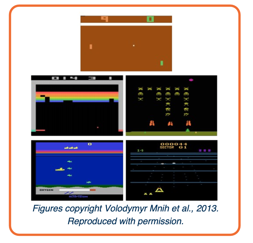
Deep Q-learning assumes a parameterized Q function that is optimized to match the optimal Q function, from a define state of $\{ (s,a,s’,r)_i \}^N_i$
The simplest example of such a parameter network, is a linear Q-network with one network vector and a Bias
\[Q(s,a;w,b) = W_a^T s + b_a\]Alternatively, the Q-network can also be a deep neural network. $Q(s,a;\theta)$
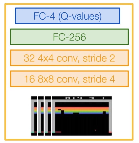
Q-network can take in RGB images, with a CNN that was used to play Atari with deep Q-learning. The input to this network is a concatenation of the last four states as RGB images, and the output is a set of key values for each possible action.
Given that we have collected N data points,
\[\{(s,a,s',r)_i \}^N_{i=1}\]The update for our Q network, will again be inspired by the recursive bellman optimality equation.
We want a Q function that satisfies the bell man optimally (Q-value)
\[Q^*(s,a) = \mathbf{E}\bigg[ \sum_{t \geq 0 } \gamma^t r_t \lvert s_0 = s, a_0 = a , \pi^* \bigg]\]We can introduce a regression objective that will minimize this mean squared error as follows:
- Predicted Q value as $Q_{new} (s,a)$
- Target Q value as $r + \gamma max_a Q_{old} (s’,a)$
Then, the MSE loss can be define as:
\[(Q_new(s,a) - (r+ max_a Q_{old} (s',a)))^2\]However, in practice, it has been observed that using a single Q-network, makes the loss minimization unstable. Instead, two copies of the Q-network are maintained at all times during training. One is called $Q_{old}$ while the other is called $Q_{new}$, which start with the same parameters.
- Freeze $Q_{old}$ and update $Q_{new}$ parameters.
- Set $Q_{old} \leftarrow Q_{new}$ at regular intervals.
In practice, we will:
- Compute the loss for a mini batch of size B
-
The forward pass will feed in the current state to the Q-network, giving us output a batch of Q-values of size B, the number of actions.
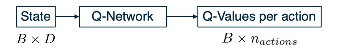
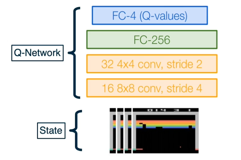
-
The loss that we will compute as an average of the MSe loss for the current batch, where the predictions are obtained by a forward pass on the $Q_{new}$ network and a forward pass on the $Q_{old}$ network.
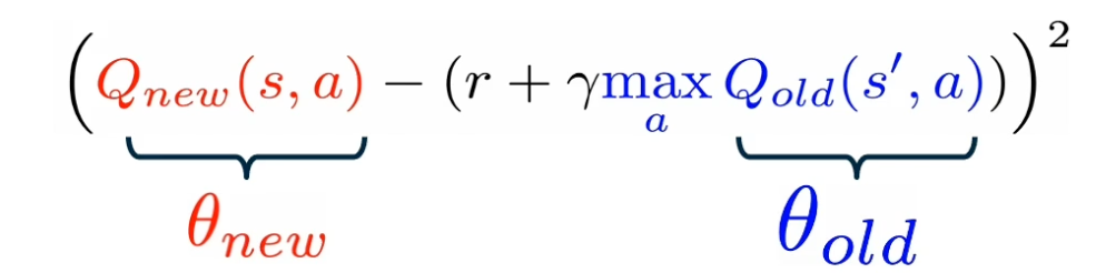
- The backward pass of gradients, will compute the derivative of this loss with respect to the new parameters $\frac{\partial L}{\partial \theta_{new}}$
We now know how to update a deep Q-network to convergence, given a fixed data set. Note that there exists an algorithm called fitted Q-iteration, whose purpose is to learn a Q-function given a fixed data set, by simply minimizing the MSE loss seen earlier. However, for our current deep Q-learning algorithm, we still haven’t answer the question of how the deep Q agent is interacting with the environment to gather experience or data? Answering this question will reveal the most challenging aspects of reinforcement learning.
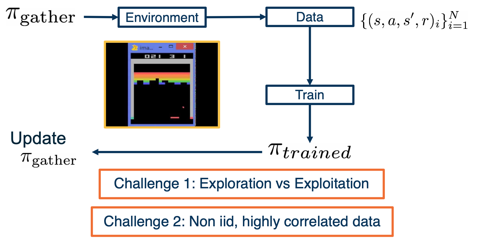
Let’s imagine that we start with a random data gathering policy called $\pi_{gather}$. We will let it interact with the environment. Initially, the data collected will be random and a few data points will inform the agent, that keeping the ball in play is rewarding. We can then use the dpn update seen earlier, to update our Q-network and obtained a greedy policy with respect to this Q-network, and we can called it $\pi_{trained}$. Now that we have a better policy that the one we started with, it is natural to also start collecting data with these better policy, i.e update $\pi_{gather}$. With this thought experiment, we have come up with our first naive strategy for interacting with the environment to collect data.
However, this is challenging because firstly, we are always updating the $\pi_{gather}$ policy with the greedy $\pi_{trained}$, it will not have incentive to explore other less rewarding states, that may eventually lead to an overall higher reward.
Secondly, if we are setting a policy with data, and then gathering data with this new policy. The data naturally will be biased by the policy, creating a feedback loop that the data will consist of only states that the policy currently believes to be rewarded. This means that the data set will no longer be i.i.d (linearly independently distributed ) but highly correlated.
Exploration Problem
Now that we know that setting the data gathering policy to be the same as the greedy train policies is a bad idea, let’s look at how the deep Q-learning algorithm solves this first challenge.
In order to always have some probability of exploration, the following $\epsilon$ greedy strategy is used for data gathering
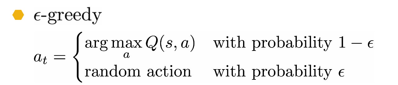
Where a random action is chosen with a typically small epsilon probability and hte greedy action is selected otherwise.
Correlated Data Problem
For the second challenge, we know that if we let our data to be highly correlated, the gradients we will obtained will have higher variance and led to inefficient training. To further elaborate on this issue, consider the one D environment that we saw with a discount factor $\gamma =1$:
If the best strategy started off by going to the right endpoint, achieving the plus one reward, the data gathering policy will then be dominated by trajectories going to the right. And even if by random chance the policy ends up reaching, the left endpoint due to exploration, the amount of data collected for the right end point will dominate the gradient update step and will prevent any changes to this sub optimal strategy.
In order to address this, deep Q-learning employs an experienced replay buffer, which is a queue of past experiences from which a mini batch is randomly sampled. The buffer is a finite size and older sample are discarded in favor of new ones. In practice, increasing the size of this buffer, will lower the correlation between data points sampled in a mini batch.
- A replay buffer stores transitions $(s,a,s’,r)$
- Continually update replay buffer as game (experience) episodes are played, older samples discarded
- Train Q-network on random minibatches of transitions from the replay memory, instead of consecutive samples
Larger the buffer, lower the correlation.
Now, we have all the tools at hand to understand the original deep Q-learning algorithm as it appeared in this paper titled playing Atari games with deep RL.
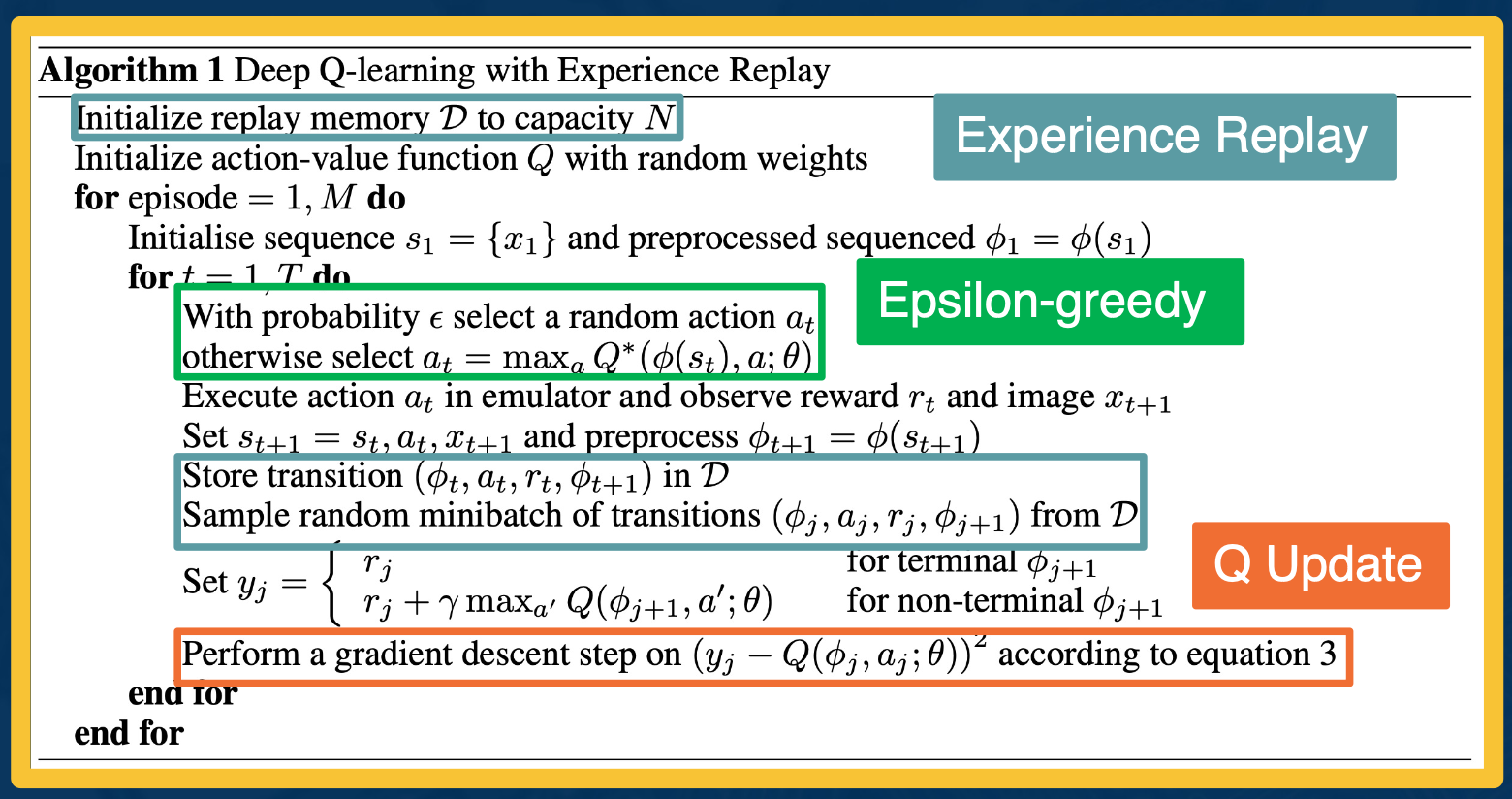
The algorithm boils down to three key mechanisms, the epsilon greedy data gathering policy in green, the experience replay buffer to store transitions in blue, and the Q-network update step in orange.
Policy Gradients, Actor-Critic
Among the types of methods using RL value based methods learn q functions, while model based methods learn the transition and reward function. In the end, both these methods provide an optimal policy that is used to perform a task with high reward.
Policy based methods on the other hand directly parameterize a policy and optimize it to maximize returns.
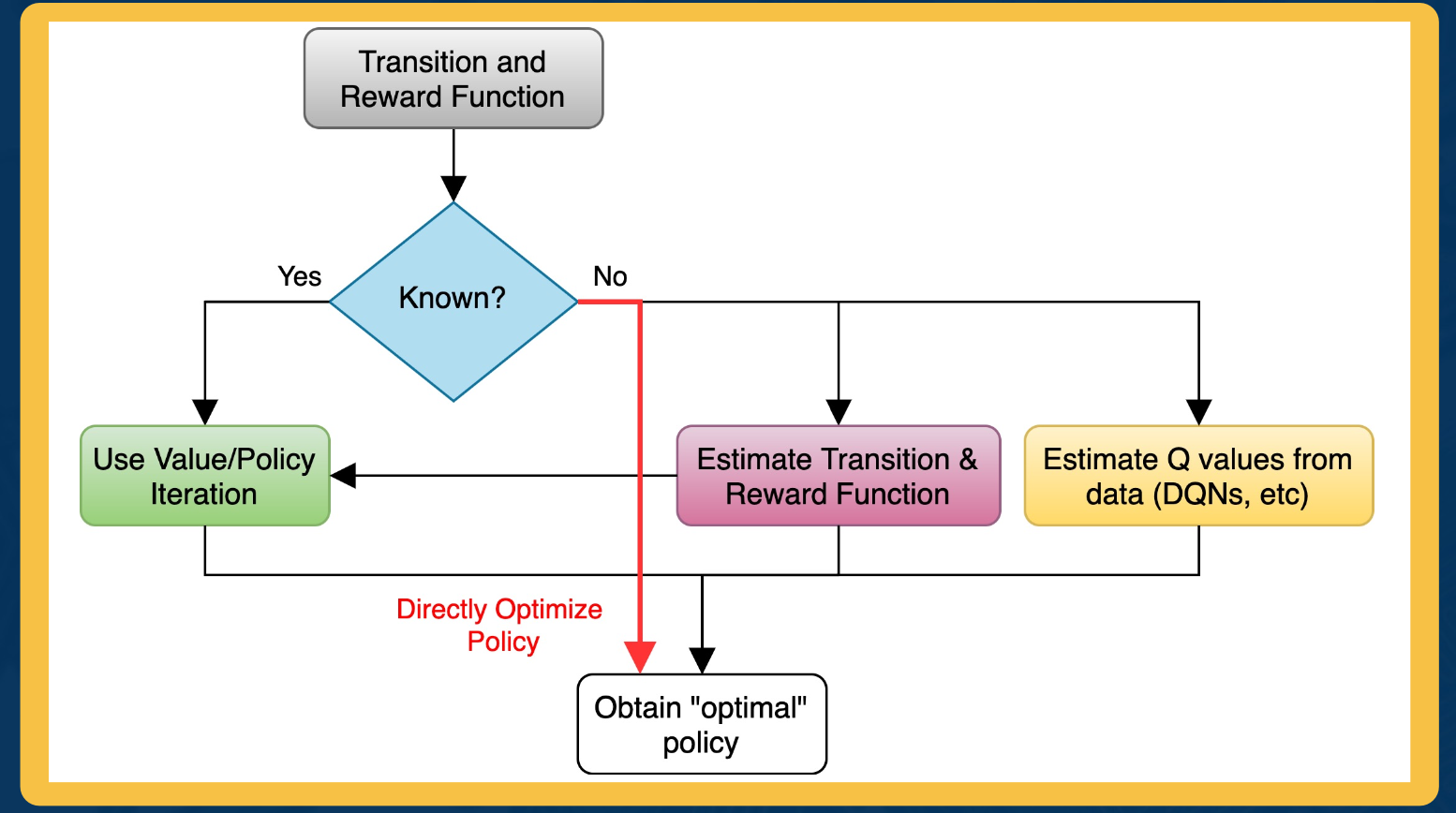
Our classes of policies will be parameterized functions that map states to actions
\[\pi_\theta (a \lvert s) : S \rightarrow A\]$\theta$ can be parameters of linear transformation, deep network etc.
The objective function $J$ measures the performance of an input policy $\pi$ as the sum of rewards over a finite time horizon T. For this lecture, we will assume that the discounting factor of gamma is one and excluded from the objective function due to the episodic or finite nature of our trajectories.
\[J(\pi) = \mathbf{E} \bigg[ \sum_{t=1}^T R(s_t,a_t) \bigg]\]Now, we can translate the original definition of optimal policy which involve this abstract maximization over all possible policies into a maximization over all parameter values $\theta$.
We will also write our objective as $J(\theta)$ instead of $J(\pi)$, as the parameters $\theta$ fully described the policy.
Policy Gradient: Loss Function
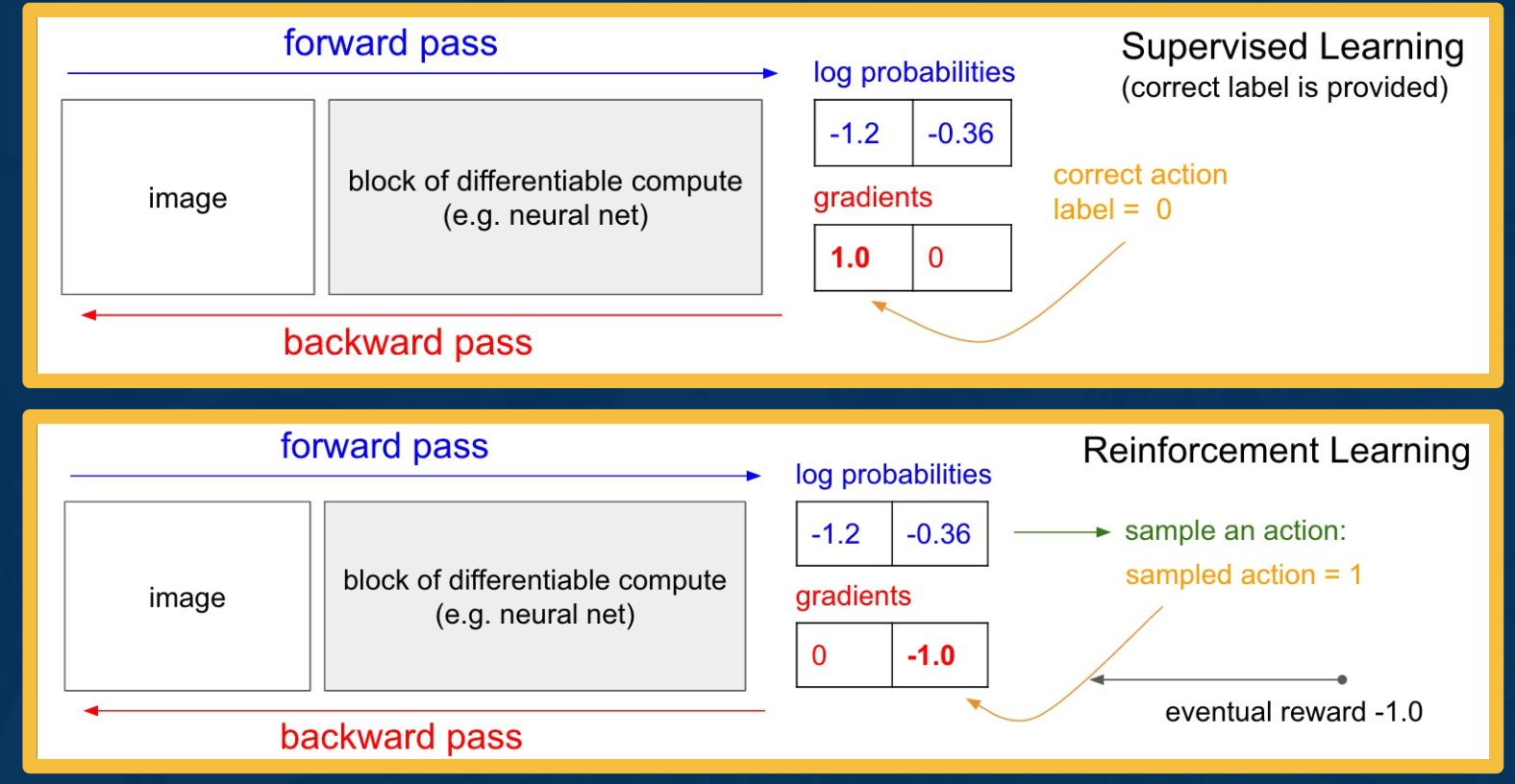
Let’s first look at an intuitive explanation of how an RL algorithm will define the gradient update step for such a policy. Recall that in supervised learning specifically, image classification, a neural network comprised of differentiable blocks used to process an image in the backward pass and produce log probability of classes.
The backward pass then propagate its gradients of the loss with respect to the parameters for each parameter in the differentiable block. Due to the presence of supervision in the form of the correct label, or let’s say the correct action, the loss can be used to maximize the log probability of the correct action.
In reinforcement learning, a parameterized policy will have a similar neural network that takes an input, the RGB image of the environment state and computes log probabilities of every action. Further, an action must be selected by sampling from this categorical distribution, and due to the fact that the reward is only provided as feedback for the selected action. A simple strategy can be to increase or decrease the log probability of the chosen action depending on the sign and magnitude of the reward obtained for selecting that action.
Gathering Data/Experience
With this intuition at hand, we will soon derive the formal policy gradient update step.
Before looking into that, let us first look at the data gathering phase of such policy based algorithms. First, let us define a finite trajectory $\tau$ are the sequence of state and actions from time steps $0 \rightarrow t$.
\[\tau = (s_0, a_0, ... , s_T, a_T)\]The probability of $\tau$ given a policy $\pi_\theta$ which is also written as $p_\theta (\tau)$ is simply the probability of the sequence of state and actions and this probability can be broken down into the probability of each state or actions given previous states or actions resulting in this expression.
\[\begin{aligned} \pi_\theta(\tau) &= p_\theta (\tau) \\ &= p_\theta (s_0, a_0, ..., s_T, a_T) \\ &= p(s_0) \prod_{t=0}^T p_\theta (a_t \lvert s_t ) \cdot p(s_{t+1} \lvert s_t, a_t) \end{aligned}\]Further, we will write our objective as finding the parameters $\theta$ that maximizes the expected sum of rewards over trajectories $\tau$
\[argmax_\theta \mathbf{E}_{\tau \sim p_\theta (\tau) [R(\tau)]}\]Thus,
\[\begin{aligned} J(\theta) &= \mathbf{E}_{\tau \sim p_\theta (\tau) [R(\tau)]} \\ &= \mathbf{E}_{a_t \sim \pi (\cdot \lvert s_t), s_{t+1} \sim p(\cdot \lvert s_t, a_t)} \bigg[\sum_{t=0}^T R(s_t,a_t)\bigg] \end{aligned}\]Now, our strategy for gathering data is going to be simple in comparison to what we saw in deep q learning.
We simply need to collect a small batch of trajectories using the current $\pi_\theta$ which can be used as a sample based approximation of our reward objective.
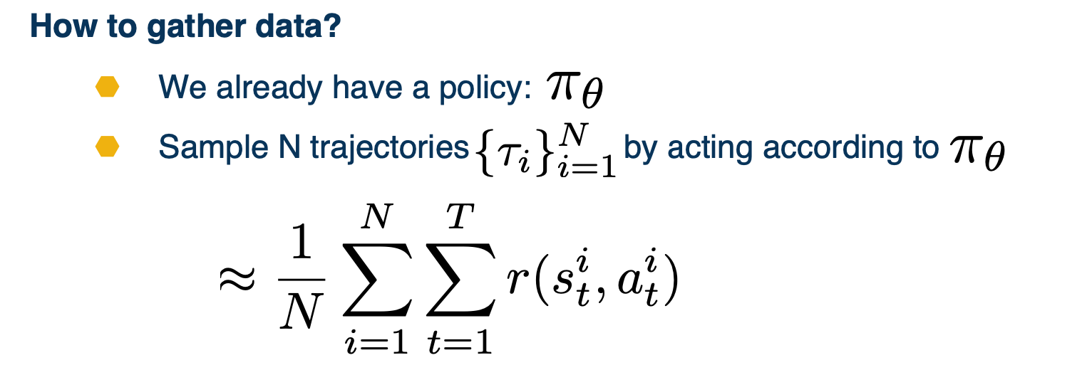
The REINFORCE Algorithm
So far, we have seen how to gather data with the current policy parameters $\theta$, and an intuitive explanation for what the policy update step will look like. What we have described so far are the components of a policy gradient algorithm, known as reinforce. This algorithm performs three tasks at each iteration, gathering data with the current policy, computing the policy gradient update and taking a gradient step to obtained the policy parameters for the next iteration. Let us now fill in the missing piece of the algorithm which is the exact expression for the policy gradient.
Deriving The Policy Gradient
Our goal is now to derive the gradient of our objective $J$ with respect to the policy parameters $\theta$. We will write first, the definition of our objective as the expected sum of rewards over trajectories $\tau$, then we can write the expectation as integral of probability density $\pi(\tau)$ and exchange the gradient and integral operator.
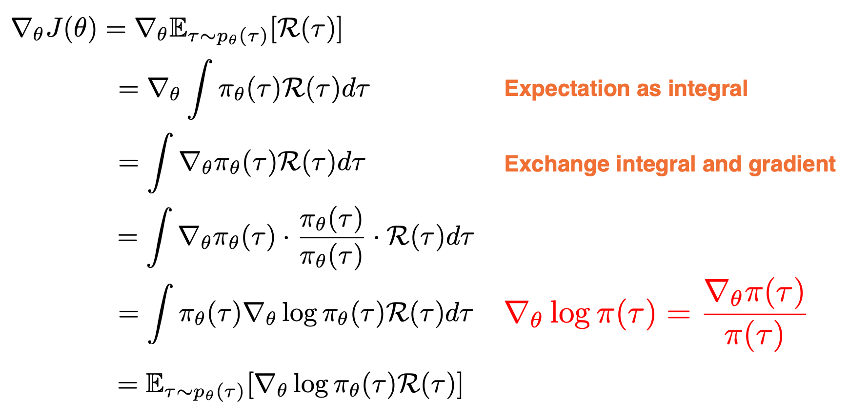
Now, we just multiply and divide the probability density $\pi(\tau)$ in order to apply a relation known as the log derivative trick, which simply uses uses the fact that the derivative of the log of a function is $\triangledown_\theta log \pi(\tau) = \frac{\triangledown_\theta \pi (\tau)}{\pi(\tau)} $ which now appears in the above expression. Substituting this ratio, we now obtained an integral of a probability density $\pi$ and some other terms. This integral can now be written as an expectation over probability density $\pi$ with the remaining terms kept the same. We started out in the second line with the gradient of an integral, but we cannot compute because we do not know the integral expression in closed form. However, what we have in the last line is an expectation of some function, which can be approximated with finite samples of trajectories gathered using $\pi$.
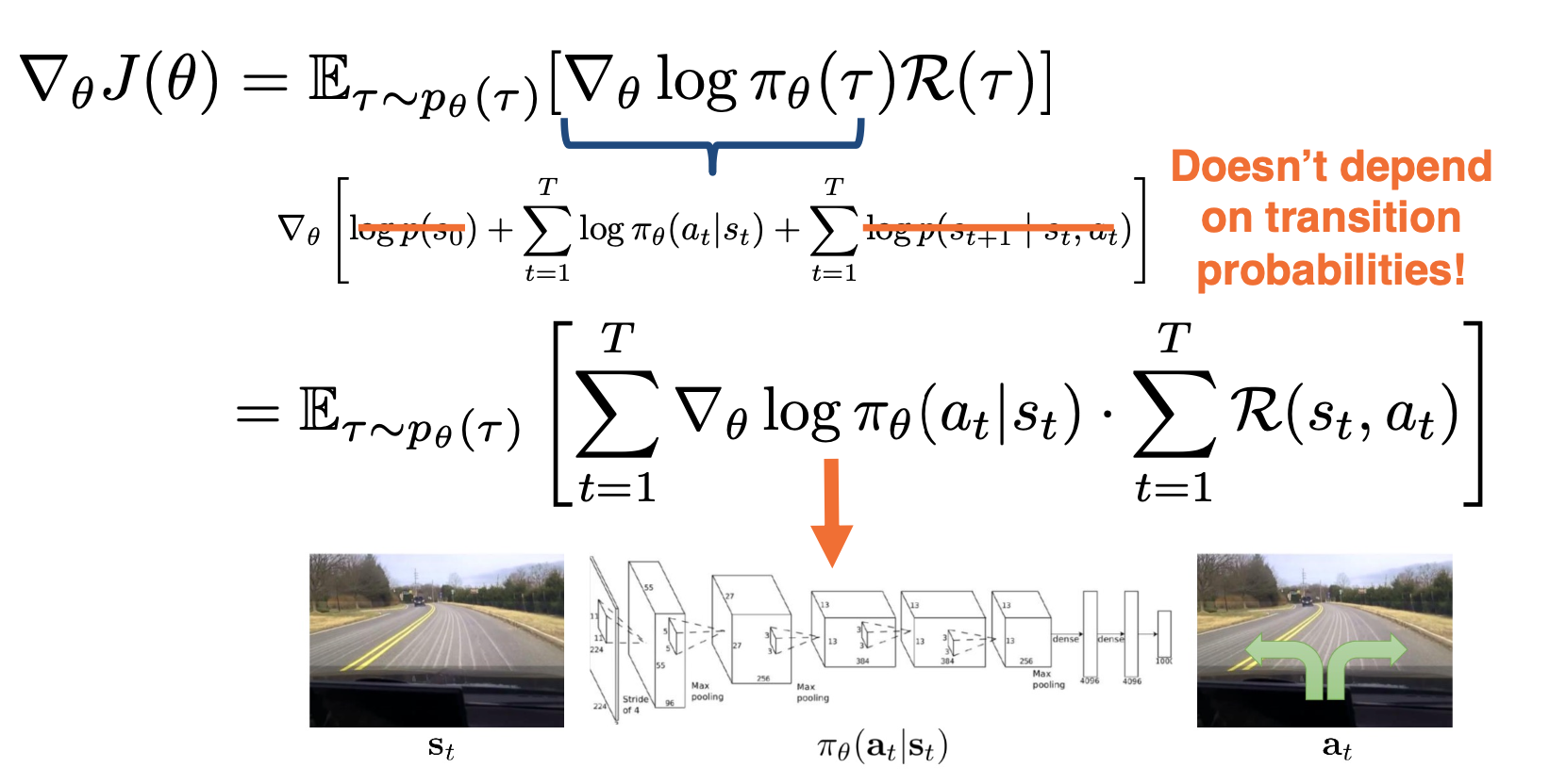
Now, we must compute the expression inside the expectation. Recall that with our definition of trajectory $\tau$, we can expand it again into a sequence of states and actions. Resulting in three types of terms that depend on the initial state distribution, the actual distribution of $\pi$ and the transition distribution. We can discard the first and the last terms as they do not depend on $\theta$ when taking the gradient shown outside. The final expression now involves the gradient of log probabilities of individual actions, which we can obtain with a simple forward pass for policy neural network at each state. The sum of these gradients is now greater with the total reward of the trajectory on the right, implying that the gradient update will push the probability of the chosen actions ot be either higher or lower depending on the sign and magnitude of the total reward for the trajectory. This is the true essence of trial and error. Only after attempting a sequence of actions will the policy know the payoff of those actions.
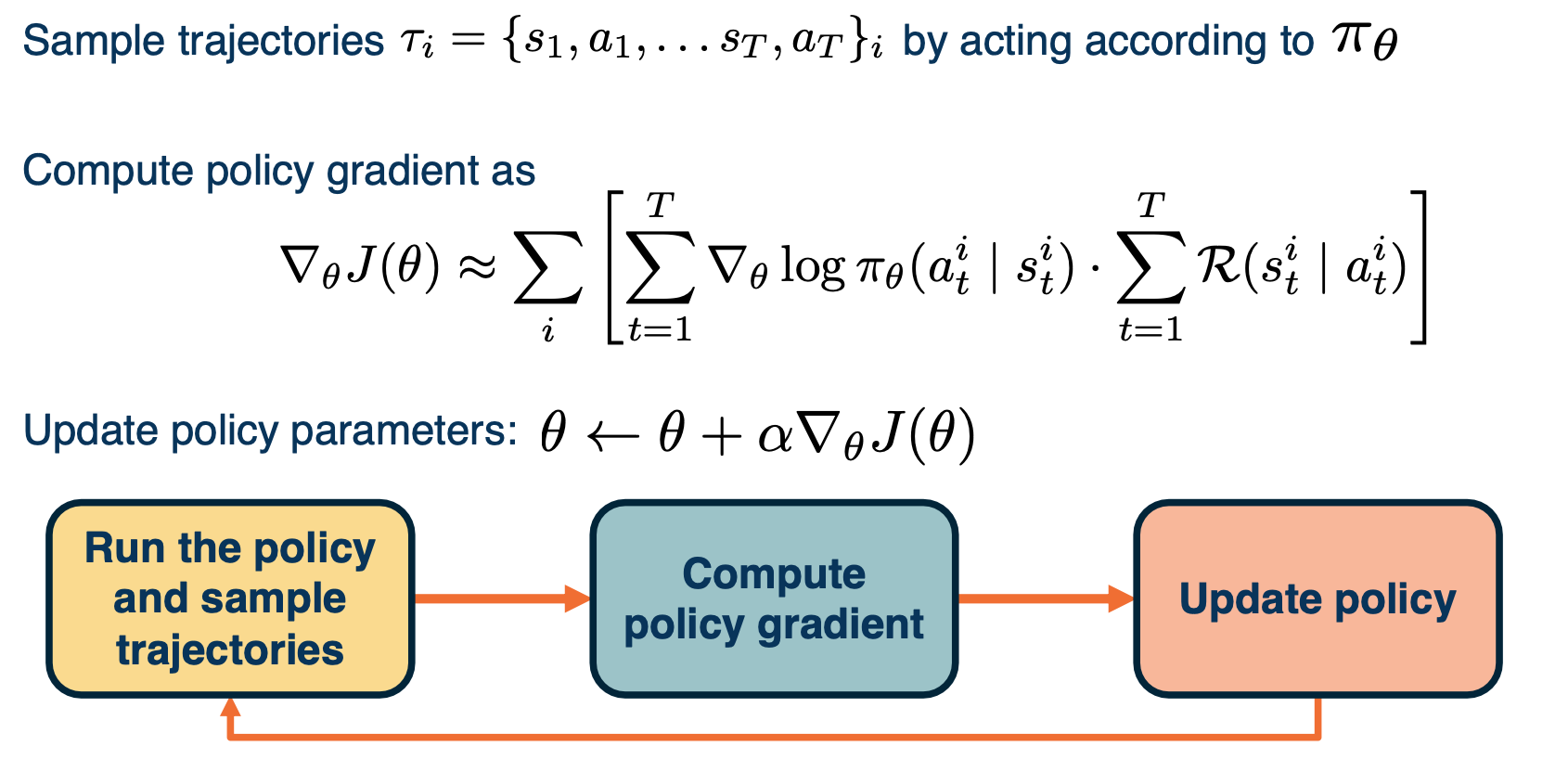
Drawbacks of Policy Gradients
The gradient update expression of this algorithm either increases or decreases the likelihood of a sequence of actions depending on the reward outcome for the entire trajectory. This means that we cannot assign credit to any particular set of actions that were good or bad. Instead, we are left with a coarse level feedback for the entire sequence of action taken.
With this credit assignment problem, new variants of this algorithm have been proposed that aim to reduce variance of policy gradient updates. The key idea behind these variations is that subtracting some baseline b shown in red below, that does not depend on actions will preserve the mean of the gradient expectation while possibly reducing the variance for specific choices of B.
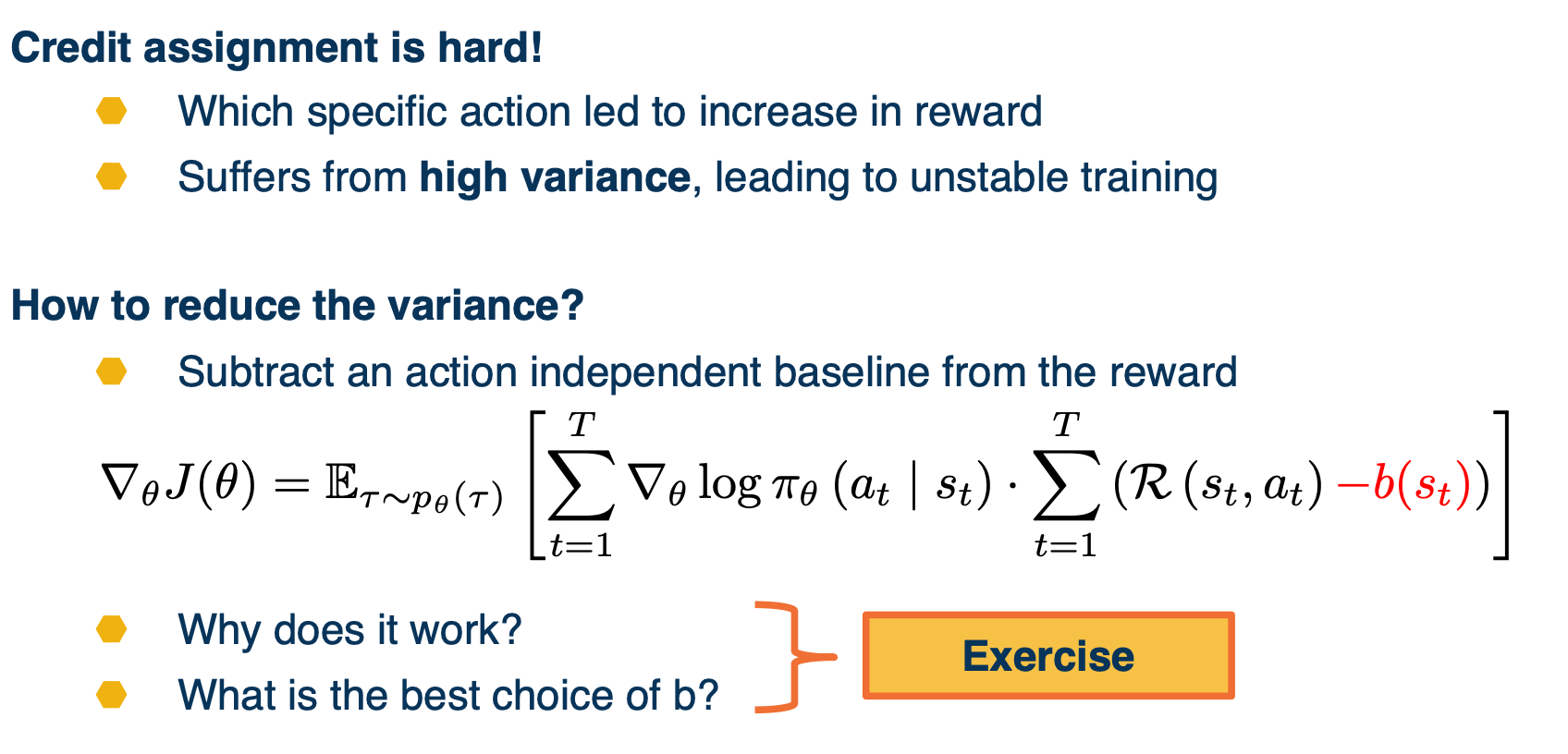
Policy Gradient Variants
The different choices of this baseline have resulted in two important variants of the policy gradient algorithm. The first is known as the actor-critic algorithm that replaces rewards with the Q function of the policy that is learned from data. The second algorithm is known as advantage actor-critic that substitutes the reward with the advantage of the policy. It is defined as the Q function minus the V function.
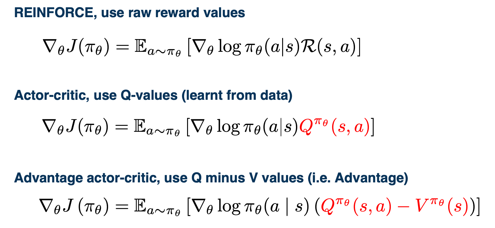
Lesson 18: Unsupervised and Semi-Supervised Learning
Readings
None!
Introduction
Comparing with the traditional way of machine learning, there is a deep learning equivalent for each of them.
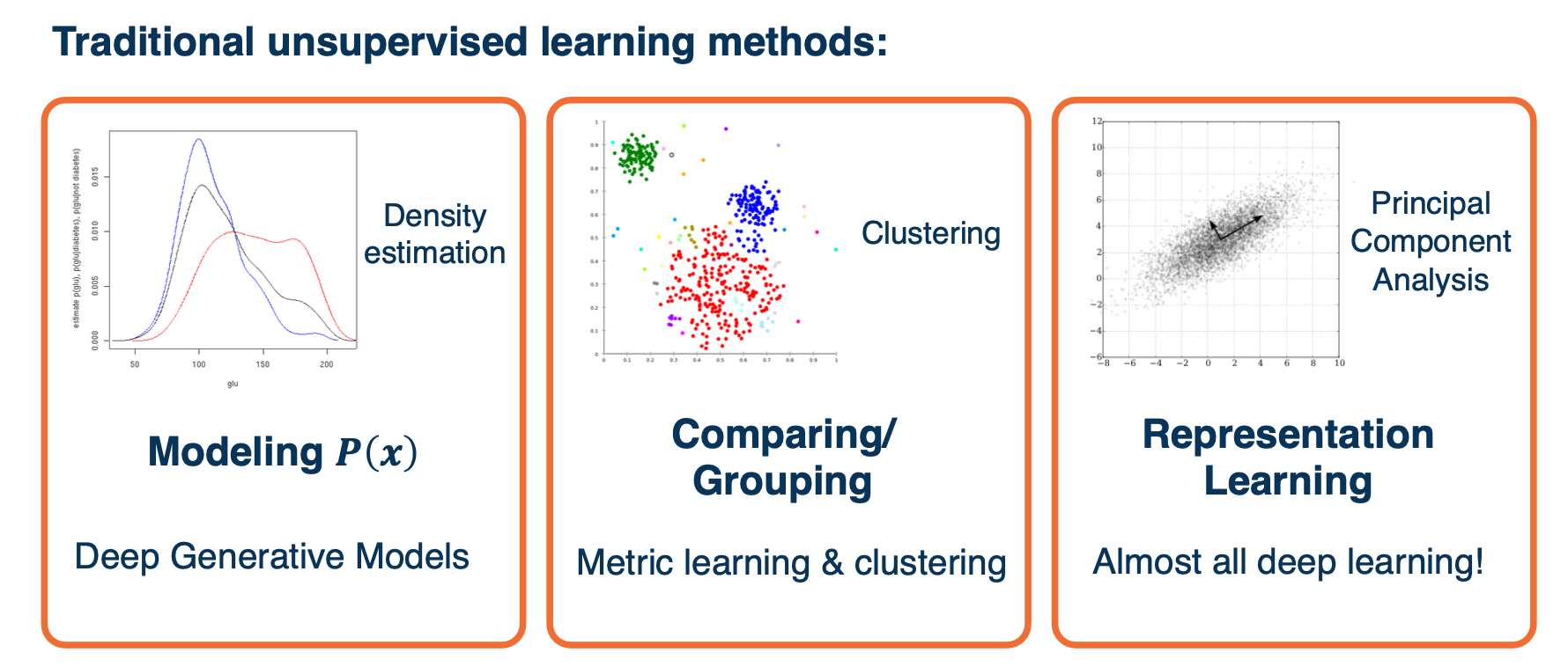
For this lesson, we will mainly focus on the representation learning part.
Dealing with unlabeled data? When we only have unlabeled data though, it is not clear what to do. There are several different considerations that we might have.
- Loss function (especially for unlabeled data)
- Optimization / Training procedure
- Architecture
- Transfer Learning
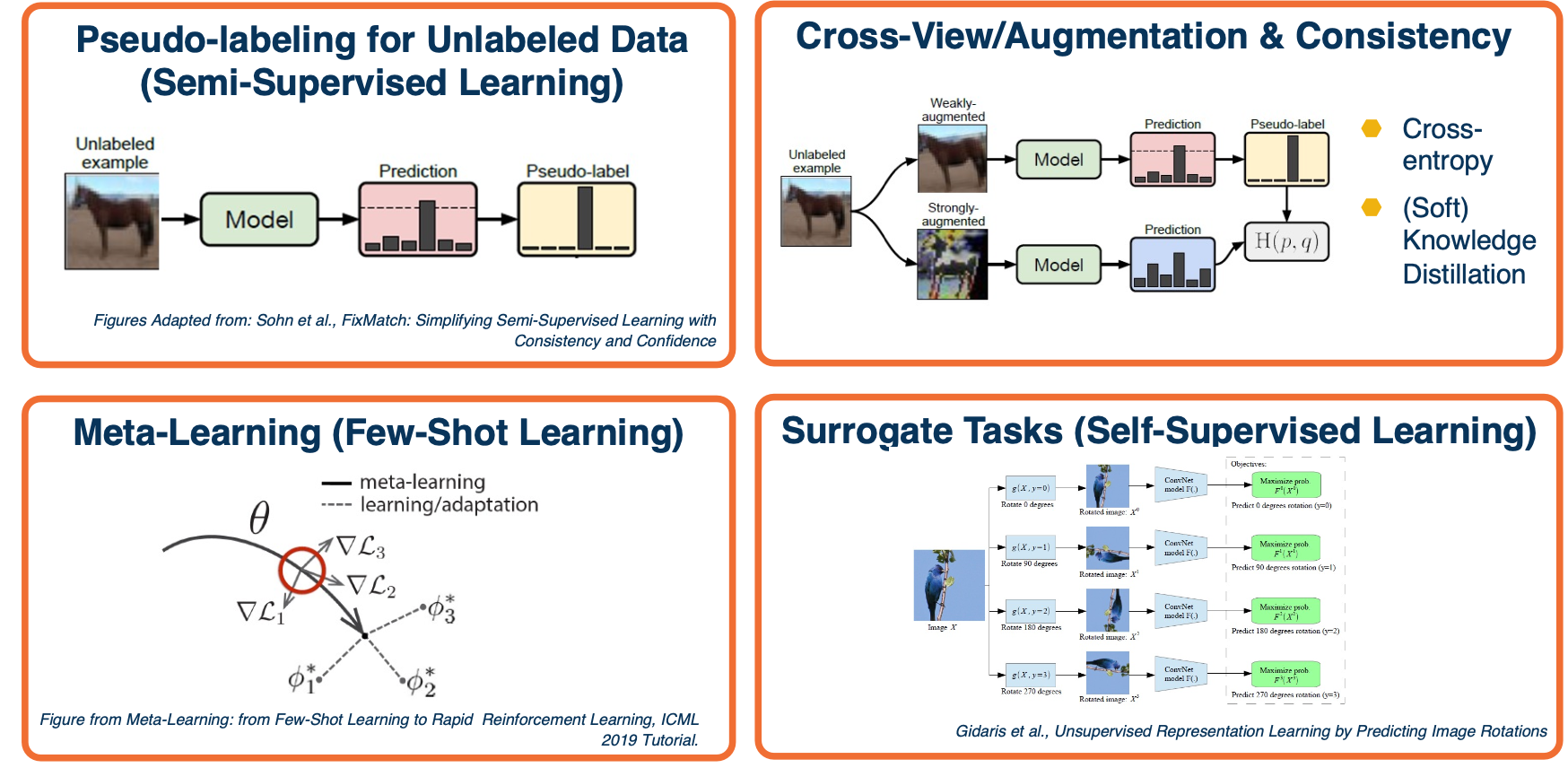
The above image shows the common ideas that keep occurring to solve these unlabeled data problem.
Semi-supervised learning
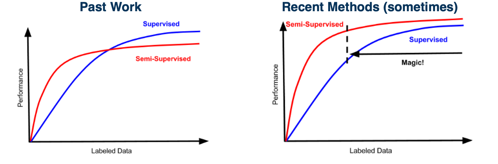
- It is often much cheaper to get large-scale unlabeled datasets
- Ideally would like to improve performance all the way to highly-labeled case
There are also old ideas:
- Simple idea: Learn model on labeled data, make predictions on unlabeled data, add as new training data, repeat.
- Combine idea with co-training: Predicting across multiple views
In a deep learning context, we can just train as normal omn the labeled data using losses such as cross entropy, and then we can perform the pseudo-labeling approach across multiple views across the image.
Pseudo-Labeling
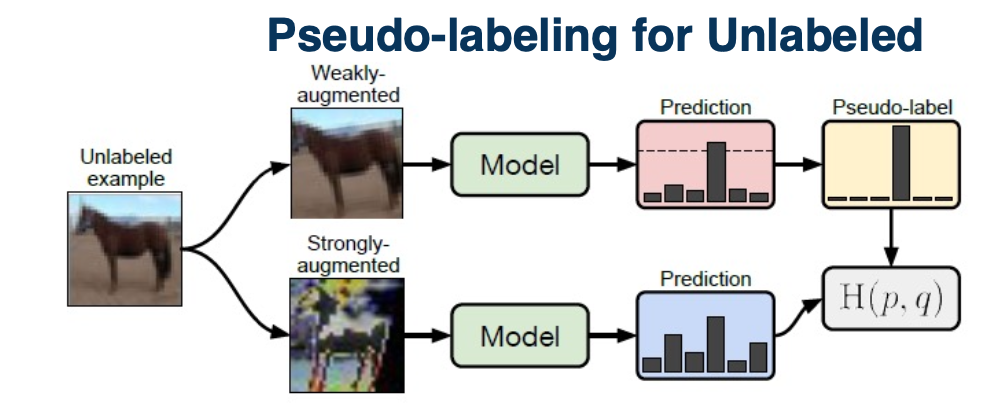
We can take an unlabeled example and perform augmentation on it. Specifically two types of augmentation, a weak type and a strong type. On the weak type, we just apply the model and get predictions and then threshold the examples by confidence. On the strong augmentations on the bottom, we will make it much more challenging for the model, and that is actually what we are going to use for backpropagation. We will use the weak version as the ground truth to train the bottom branch. This is an algorithm called fixmatch. This has proven to be extremely effective in the semi-supervised learning context.
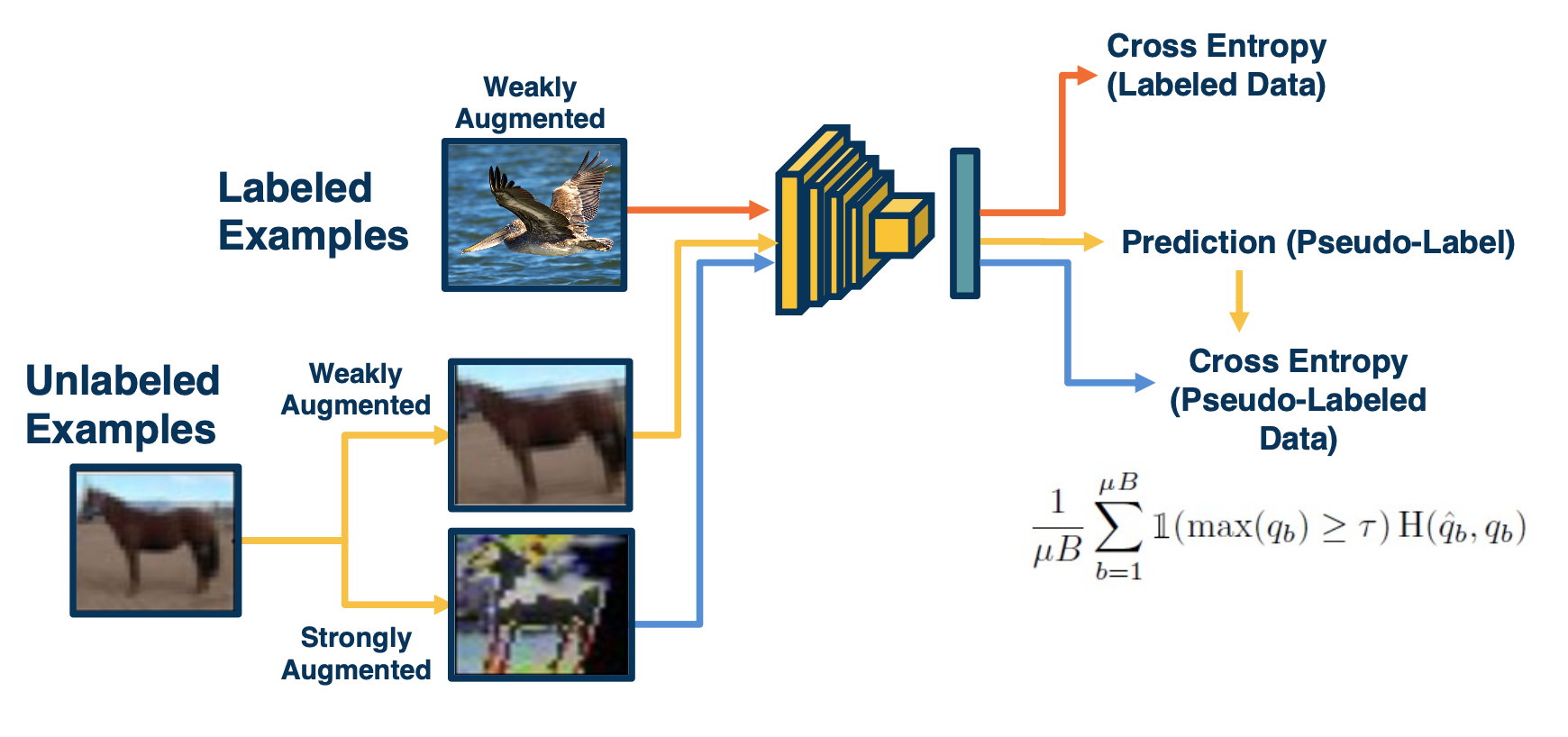
The beauty of deep learning is we do not actually have to do this in stages, we can have this entire pipeline trained in an end to end manner. Specifically, we can have the mini batch consist of both labeled and unlabeled examples. For the labeled part of the mini batch, it goes through the traditional pipeline. We will extract features, make predictions and then use cross-entropy loss because we have ground truth labels annotated by humans. For the unlabeled examples, we will apply the two types of augmentations, do feature extraction and prediction and then use the predictions obtained on the weakly augmented labeled data, not in its own loss function but really as ground truth for the loss from the strongly augmented data.
The equation above is what the loss function looks like for the unlabeled part.
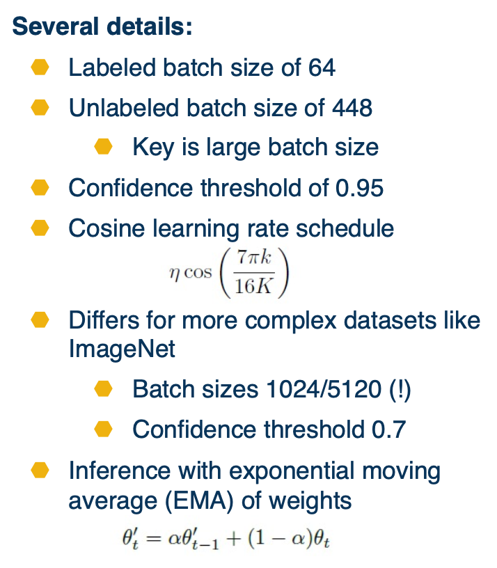
Early researchers took quite a while to get this right, the above image shows some of the important details.
There are also other newer methods as well:
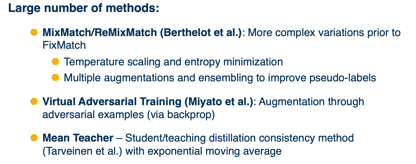
There are also other methods besides pseudo labeling such as label propagation. They allow to essentially learn feature extractors and take those extractors and apply on unlabeled data. This is similar to a clustering approach that nearby elements should be labeled similarly.
Few shot learning
In few shot learning, you have a lot of labels in a base set of categories, but very small few labels in new categories.
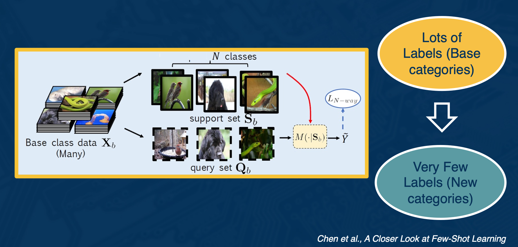
One way to do this is by fine tuning
- Train classifier on base classes
- Optionally freeze feature extractors
- In other words you are using the classifier to learn how to extract features
- Learn classifier weights for new classes using few amounts of labeled data
- If you can find the right hyperparameter you can actually do quite well.
Cosine classifier
Other than using a fully connected layer, we can use a cosine classifier
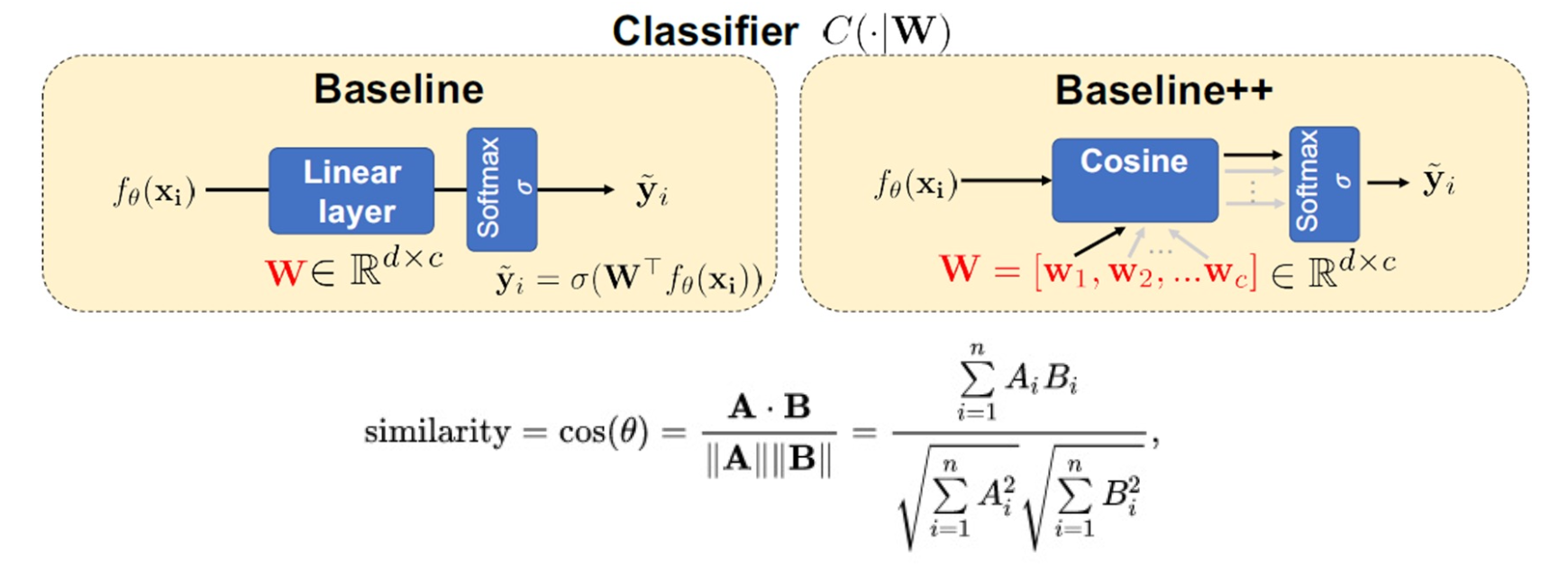
Here we still have a set of weights, but we can interpret each weight vector as as set of prototypes. That is, what the classes might look like. We perform some similarity computation between these prototypes and the query, and the output of that is also fed to a softmax.
Because we are only separating a small number of classes, this ends up working better than a normal linear layer.
Cons:
- The training we do on the base classes does not factor the task into account
- No notion that we will be performing a bunch of N- way tests
Meta Training
We take our large base dataset that has many categories, and simulate a set of smaller tasks which better mirror what will happen during testing, specifically the N-way K-short tasks, where N is the number of categories, K is the number of examples per category.
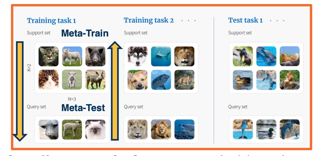
In other words, we train using the meta-train set, and we perform a meta-test and feed that gradient back as part of back propagation.
- Can optionally pre-train features on held-out base classes
- Testing stage is now the same, but with new classes.
So, what can we learn from these meta learning tasks? How do we learn a model condition on support set $M(\cdot \lvert S)$.

On the image you see what is called a matching network, which just learn a feature extractor, such that when we feed the support set into those feature extractors and extract the features and then similarly extract features for the query set, some hand coded metric actually allows you to find the most similar class for each query item. There are other types of networks such as the proto net or relation net.
We cna view this as parameterizing an actual learning algorithm itself. That is, we are taking the meta-training task 1, we have a support set and we want to perform some learning on that support set, and perform predictions on some query set.
Two approaches to defining a meta-learner:
- Take inspiration from a known learning algorithm
- kNN/kernel machine: Matching networks (Vinyals et al. 2016)
- Gaussian classifier: Prototypical Networks (Snell et al. 2017)
- Gradient Descent: Meta-Learner LSTM (Ravi & Larochelle, 2017) , Model-Agnostic Meta-Learning MAML (Finn et al. 2017)
- Derive it from a black box neural network
- MANN (Santoro et al. 2016)
- SNAIL (Mishra et al. 2018)
Meta-learner Lstm:
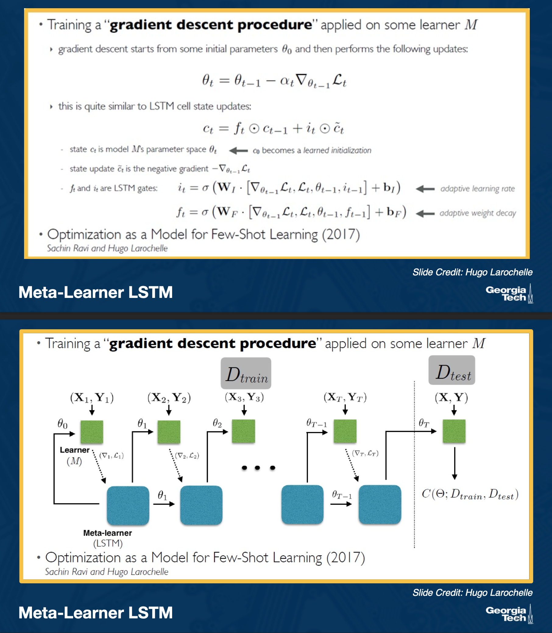
Model-Agnostic Meta-Learning (MAML)
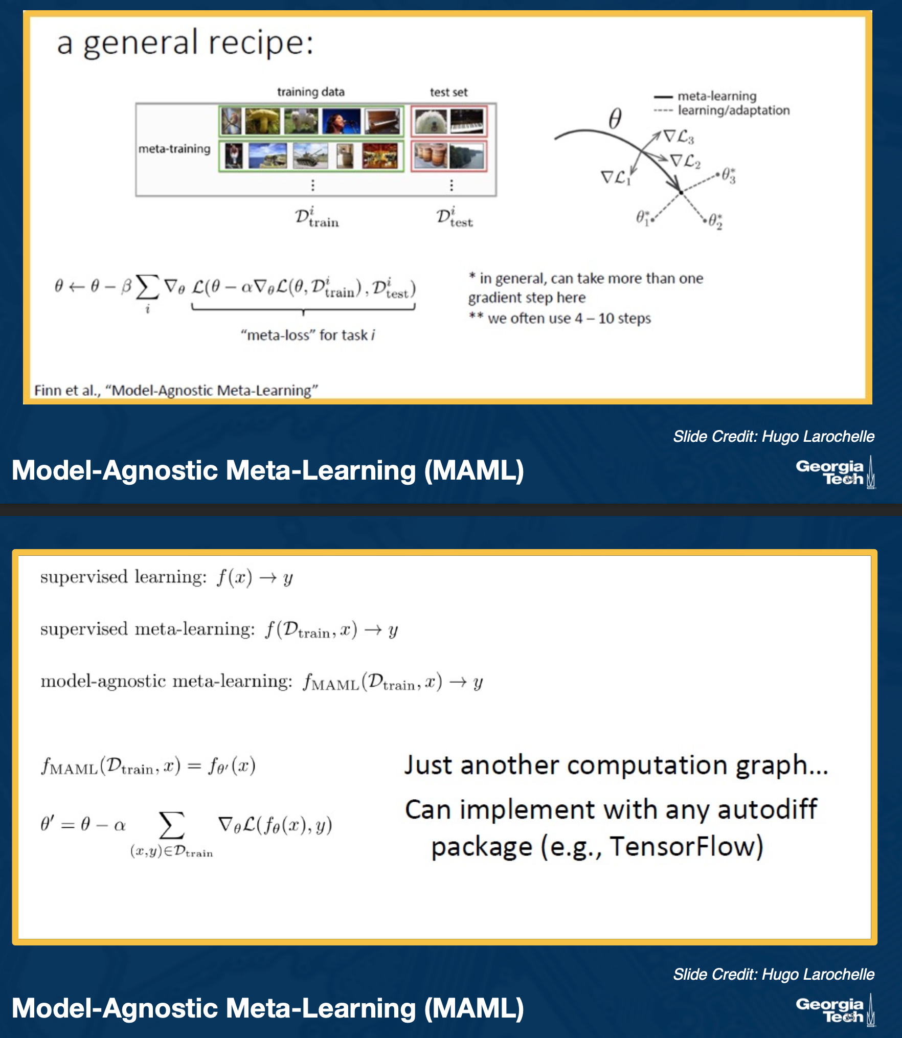
Comparison:
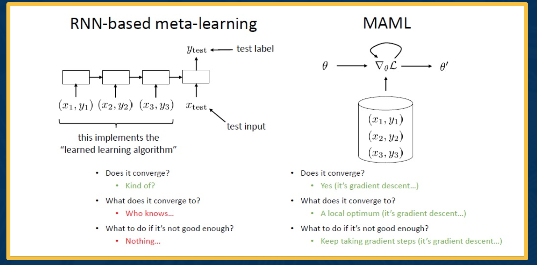
Unsupervised and self supervised learning
This is when we have no labeled data, and we are only interested to learn feature representations for downstream tasks.
Autoencoder
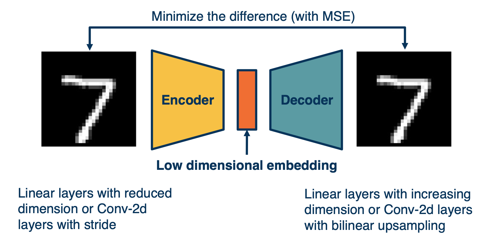
One such way is to use auto encoder, i.e to reproduce the input. and then, use the input for a classifier. This forces the neural network to learn important low dimensional features to capture important aspects of the input.
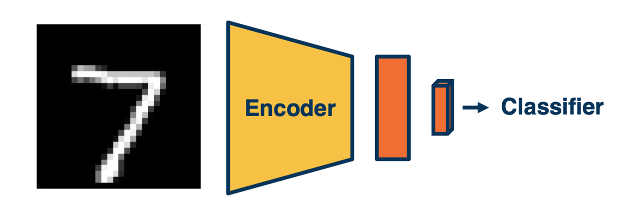
Deep clustering
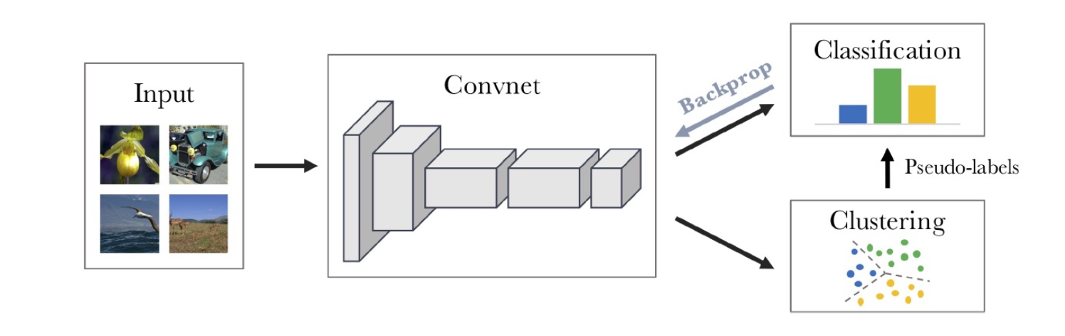
Use the outputs of the convnet and run classic clustering algorithms, and use them as labels for classifications.
Possible problems:
- Empty cluster
- Trivial parameterization
Surrogate tasks
We can also “trick” or “force” the neural network to learn feature representation, such as :
- Reconstruction
- Rotate images,predict if image is rotated or not
- Colorization
- Relative image patch location (jigsaw)
- Video: Next frame prediction
- Instance Prediction
Colorization example:
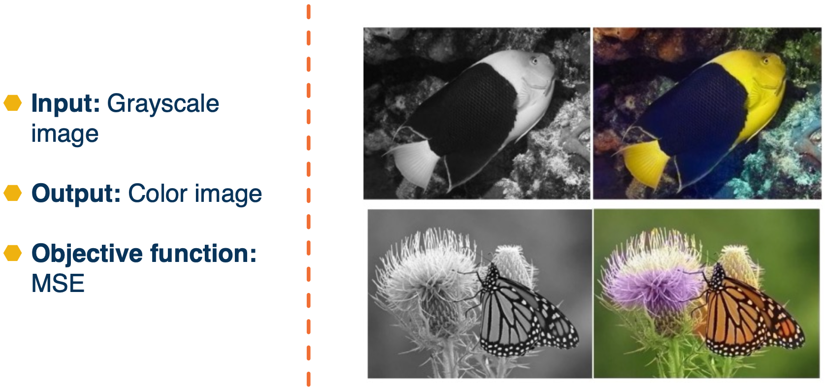
Jigsaw example:
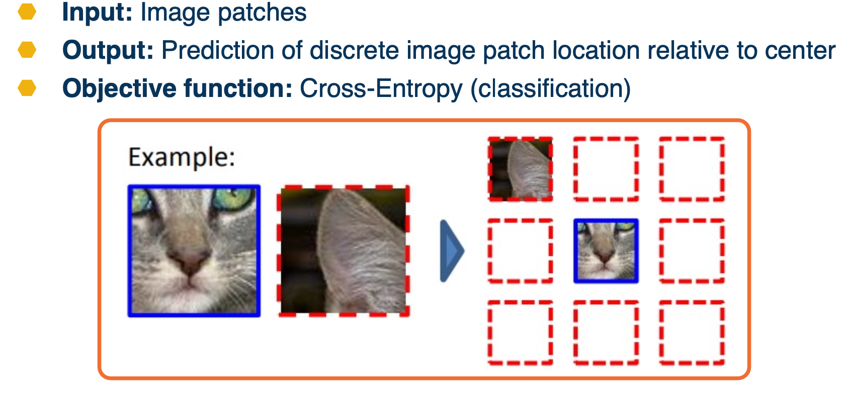
All this sounds good, but, how do we evaluate the Model?
- Train the model with a surrogate task
- Extract the ConvNet (or encoder part)
- Transfer to the actual task
- Use it to initialize the model of another supervised learning task
- Use it to extract features for learning a separate classifier (ex: NN or SVM)
- Often classifier is limited to linear layer and features are frozen
In other words, use the features learn and feed it through a simple model where you have labeled data to measure the performance.
There are other methods such as:
- Instance discrimination
- momentum encoder
- memory banks
In summary,
Large number of surrogate tasks and variations!
- E.g. contrastive across image patches or context
- Different types of loss functions and training regimes
Two have become dominant as extremely effective:
- Contrastive losses (e.g. instance discrimination with positive and negative instances)
- Pseudo-labeling (hard pseudo-label) and knowledge distillation (soft teacher/student)
Data augmentation is key
- Methods tend to be sensitive to choice of augmentation
Lesson 19: Generative Models
Readings
Generative Models Introduction
In this lecture we will focus on density estimation, that is producing a model of the probability distribution over the input space. Or in some case, we may want to just have the ability to generate samples from this distribution.
These has some history, such as Gaussian mixture models.
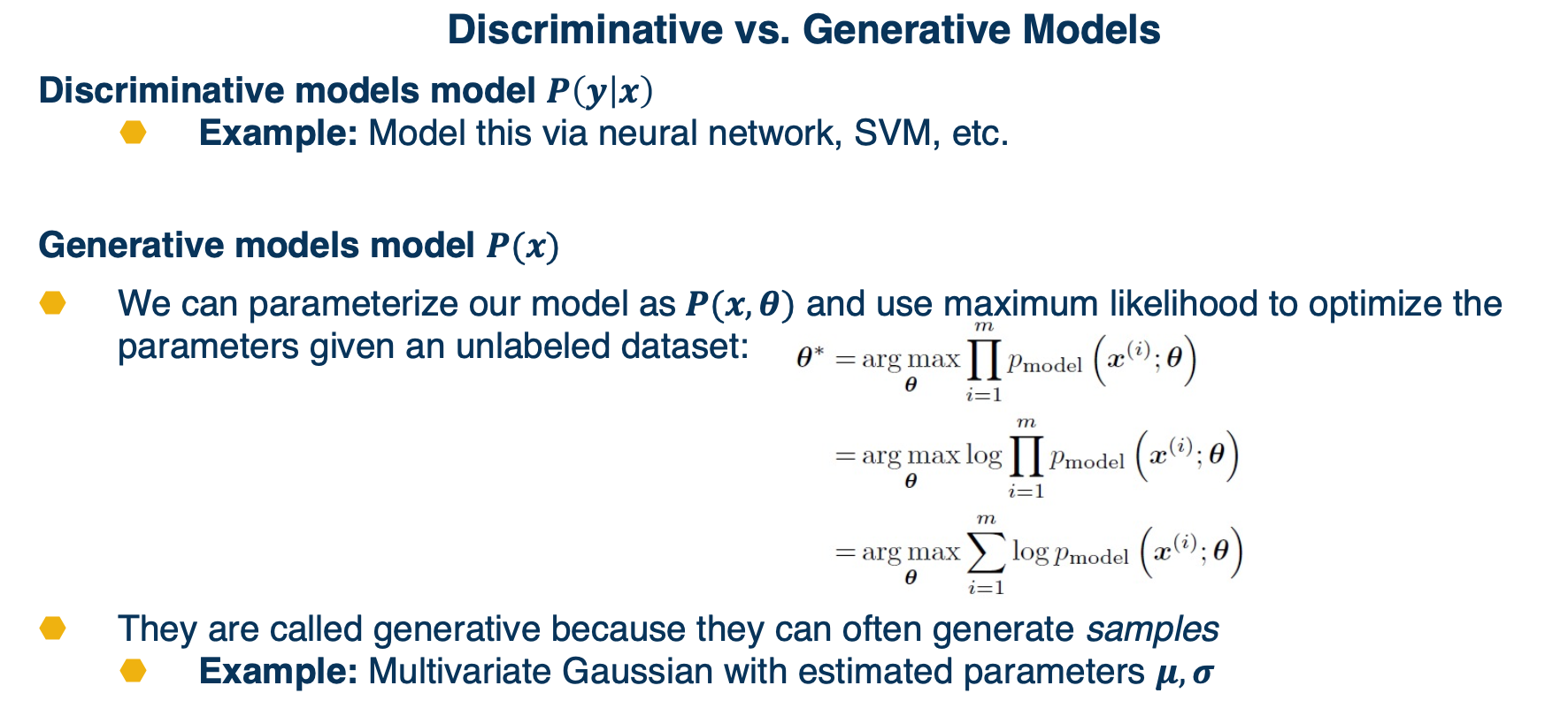
There are many various methods,
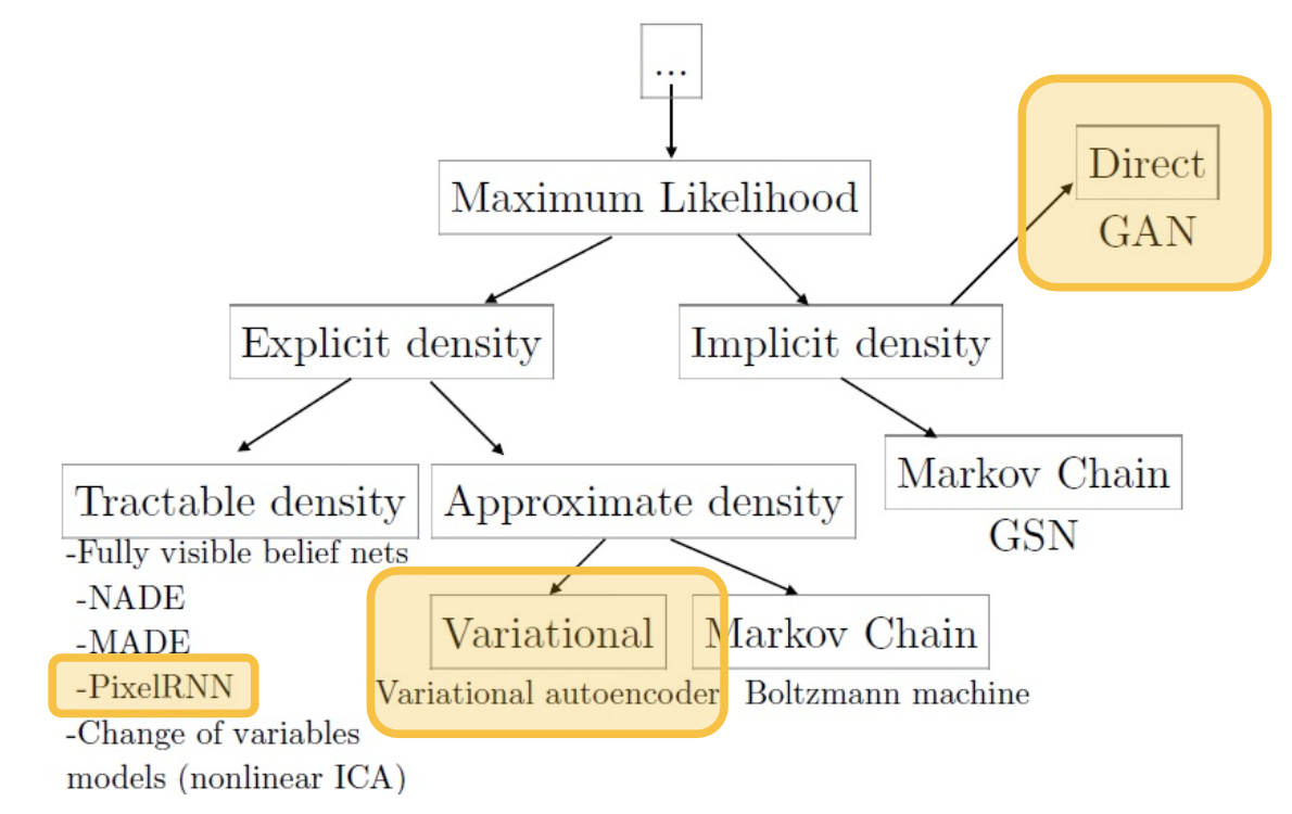
We will cover the most popular methods, highlighted in the yellow boxes.
PixelRNN & PixelCNN
We can use chain rule to decompose the joint distribution
- Factorizes joint distribution into a product of conditional distributions
- Similar to Bayesian Network (factorizing a joint distribution)
- Similar to language models!
- Requires some ordering of variables (edges in a probabilistic graphical model)
- We can estimate this conditional distribution as a neural network
Language modeling involves estimating a probability distribution over sequences of words, and we can do something similar with images:
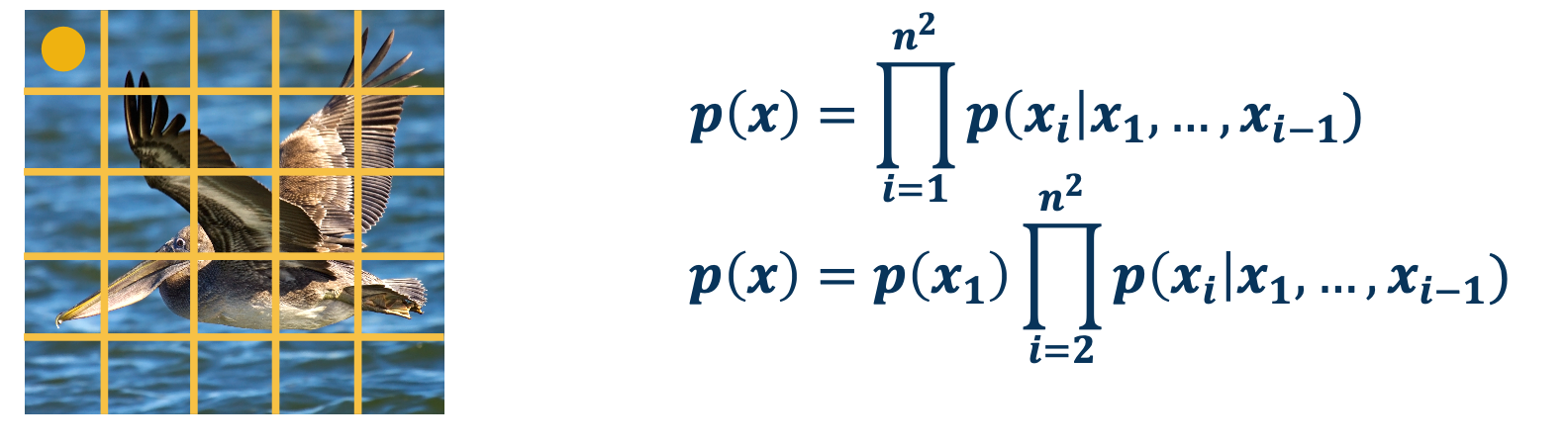
Rather than the basic unit being words, the basic units are pixels. We can factorize the joint distribution as the product of conditionals, where we define some ordering over the pixels. For example, we could start with just the upper left pixel, and have some prior probability distribution over that pixel value. We can then move to the subsequent pixels from left to right and top to bottom, we can then model the probability of x as equal to the probability of $x_1$, the upper left pixel times the probability of $x_2$ given $x_1$ times the probability of $x_3$ given $x_1$ times the rest of the product.
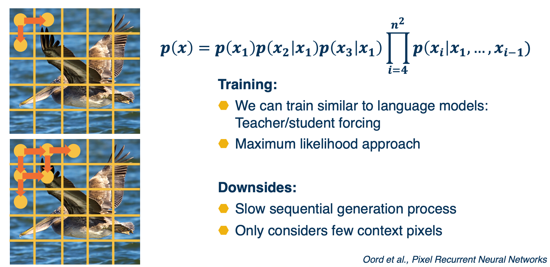
We can also use techniques such as teacher forcing, MLE approach etc. Once we have trained the model, we can actually generate new images, just sample from $p(x_1)$ that is the prediction of the model for the first pixel and then use that as input to predict the next pixels and sample from that. There is a lot of downsides to this, such as doing this sequentially in the particular order that we came up with across the entire image. This can be really slow, unlike convolution layers it is not parallelized. Also, we are only considering a few context pixels, that is given one particular pixels, we are considering a few adjacent pixels that are connected to it.
![]()
One idea is to represent the conditional distribution as a convolution, that is rather than conditional on just the adjacent pixels, we have a receptive field or a window and then we have a learnable convolution filter that output this distribution. The downside is that there’s some future pixels that is part of the convolution window that we may not know. And so we have to use things like masking in order to mask out the future pixel and only consider the previous pixel in whatever ordering that we defined here.
Generative Adversarial Networks (GANs)
Generative adversarial networks or GANS did not learn an explicit density function $p(x)$, rather they fit under the implicit density category. What that means is rather than learn a parameterized density function We will instead learn a parameterized generation process that can give us samples from the joint distribution.
We won’t have an explicit density though, to perform things like classification or things like that. But we’ll still be able to use the unlabeled data to learn how to generate new samples that fits that distribution of the unlabeled data, or even learn features that might be good for downstream tasks.
Implicit generative models do not actually learn an explicit model for $p(x)$ Instead, learn to generate samples from $p(x)$
- Learn good feature representations
- Perform data augmentation
- Learn world models (a simulator!) for reinforcement learning
How?
- Learn to sample from a neural network output
- Adversarial training that uses one network’s predictions to train the other (dynamic loss function!)
- Lots of tricks to make the optimization more stable.
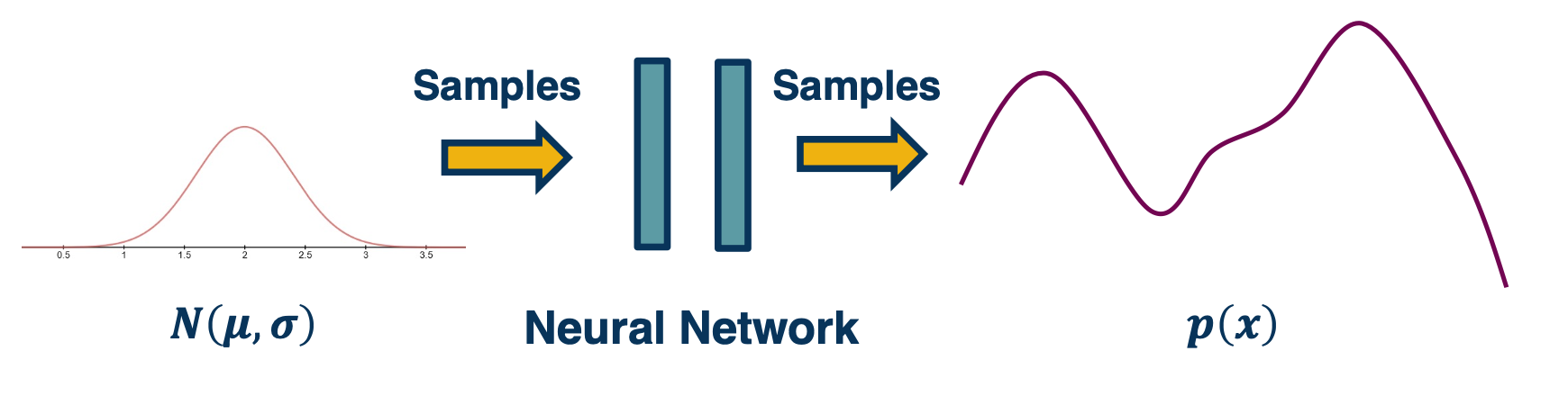
For example, we can generate random numbers then feed in with a neural network (Which can model any complex function) to generate the images.
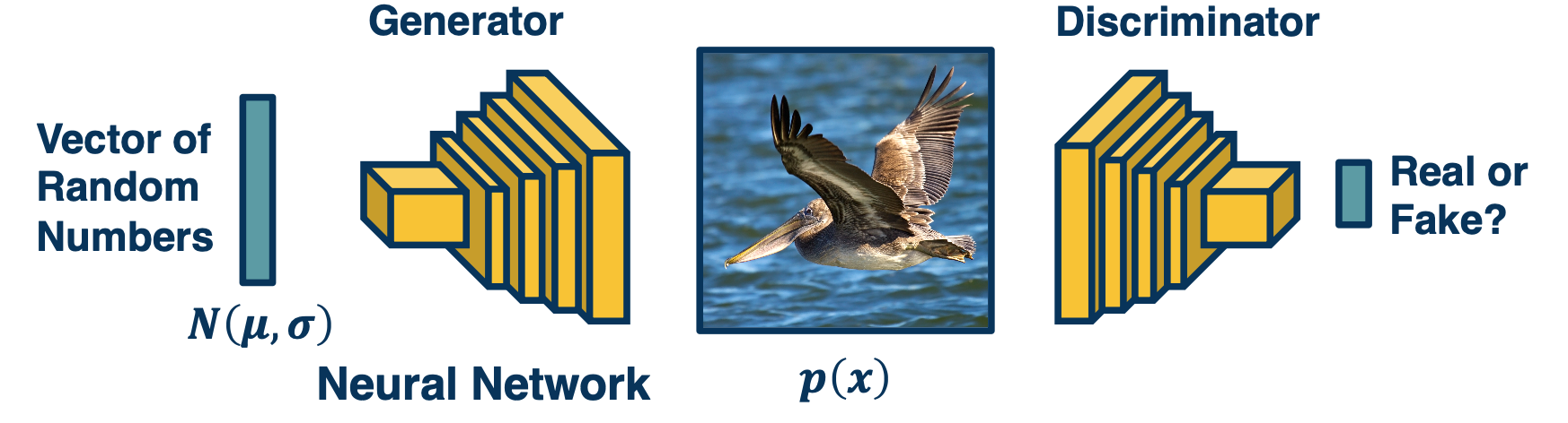
- Goal: We would like to generate realistic images. How can we drive the network to learn how to do this?
- Idea: Have another network try to distinguish a real image from a generated (fake) image
- Why? Signal can be used to determine how well it’s doing at generation
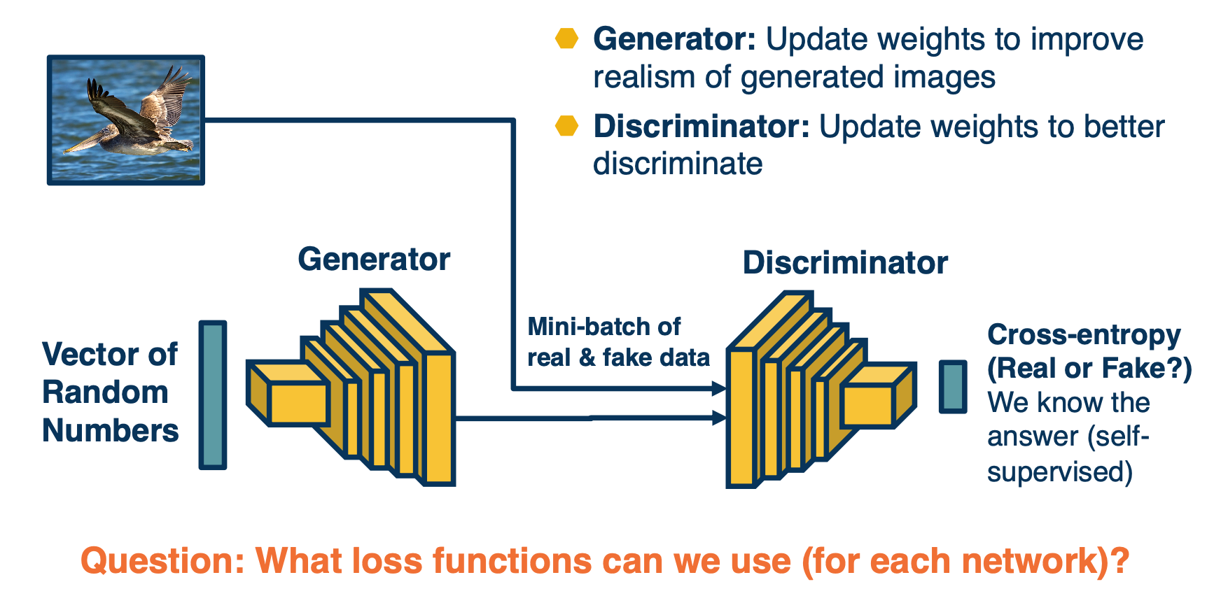
So we can just feed in at once, and train both the generator and discriminator at once. (basically try to get them to trick each other)
- Since we have two networks competing, this is a mini-max two player game
- Ties to game theory
- Not clear what (even local) Nash equilibria are for this game
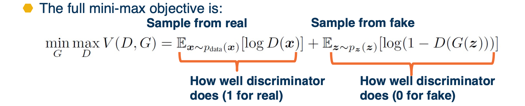
- Generator minimizes while discriminator maximizes.
- Where $D(x)$ is the discriminator outputs probability $([0,1])$ of real image
- $x$ is a real image and $G(z)$ is a generated image
- The generator wants to minimize this:
- $1-D(G(z))$ is pushed down to 0 (so that $D(G(z))$ is pushed to 1)
- This means that the generator is fooling the discriminator, i.e. succeeding at generating images that the discriminator can’t discriminate from real
- The discriminator wants to maximize this:
- $D(x)$ is pushed to 1 because $x$ is a real image
- $1-D(G(z))$ is also pushed to 1 (so that $D(G(z))$ is pushed down to 0)
- In other words, discriminator wants to classify real images as real (1) and fake images as fake (0)
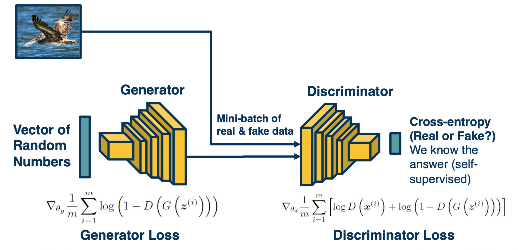
The generator part of the objective does not have good gradient properties
- High gradient when $D(G(z))$ is high (that is, discriminator is wrong)
- We want it to improve when samples are bad (discriminator is right)
The alternative objective, rather than having a minmax, we will have a maxmax:
\[max_{\theta_g} \mathbf{E}_{z \sim p(z)} log (D_{\theta_d} (G_{\theta_g}(z)))\]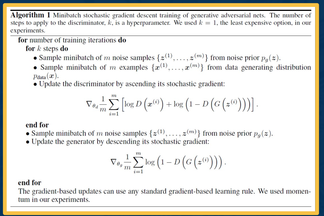
GANs are very difficult to train due to the mini-max objective
- Advancement include:
- More stable architectures
- REgularization methods to improve optimization
- Progressive growing/training scaling
Architecture guidelines for stable Deep convolutional GANs:
- Replace nay pooling layers with strided convolutions (discriminator) and fractional-strided convolutions (generator)
- Use batchnorm in both the generator and discriminator
- Remove fully connected hidden layers for deeper architectures
- Use ReLU activation in generator for all layers except for the output, which uses Tanh
- Use LeakyReLU activation in the discriminator for all layers.
For Regularization - training GANs is difficult due to:
- minmax objective - For example, what if generator learns to memorize training data (no variety) or only generates part of the distribution?
- Mode collapse - capturing only some nodes of distribution
Several theoretically-motivated regularization methods
- Simple example: Add noise to real samples!
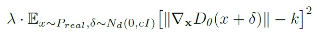
Generative Adversarial Networks (GANs) can produce amazing images!
- Several drawbacks
- High-fidelity generation heavy to train
- Training can be unstable
- No explicit model for distribution
- Larger number of extensions
- GANs conditioned on labels or other information
- Adversarial losses for other applications
Variational Autoencoders (VAEs)
Recall in our auto encoders:
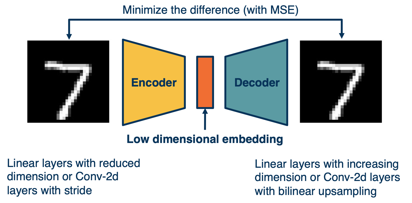
Where the input is fed through an encoder, in order to generate a low-dimensional embedding. And this low dimensional embedding or bottle neck is then used in the decoder in order to reconstruct the image.
A loss function such as mean squared error can be used in order to minimize the difference between the input and the reconstruction.
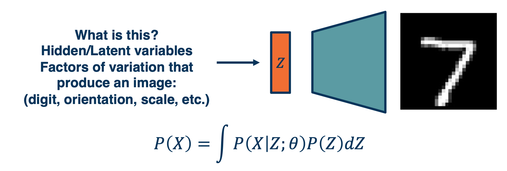
The actual bottle neck features are hidden or latent variables. What we like them to be is disentangled factors of variation that produce an image.
We can actually write down an equation for the likelihood that involves these latent variables which we call $z$, specifically we can marginalize out the $Z$. So $P(x)$ can be just the integral of $P(X\lvert Z;\theta)$, since it is the parametric model that we will use times $P(Z)$.
If we can directly maximize this, then we are essentially maximizing the likelihood and optimizing the materials, but we cannot really do this because:
- We cannot maximize this likelihood due to the integral
- instead, we maximize a variational lower bound (VLB) that we can compute.
Variational Autoencoder: Decoder
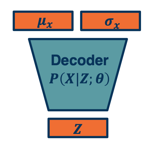
- We can combine the probabilistic view, sampling, autoencoders, and approximate optimization
- Just as before, sample 𝑍 from simpler distribution
- We can also output parameters of a probability distribution!
- Example: 𝜇, 𝜎 of Gaussian distribution
- For multi-dimensional version output diagonal covariance
- How can we maximize $P(X) = \int P(X\lvert Z;\theta) P(Z) dZ$
Variational Autoencoder: encoder
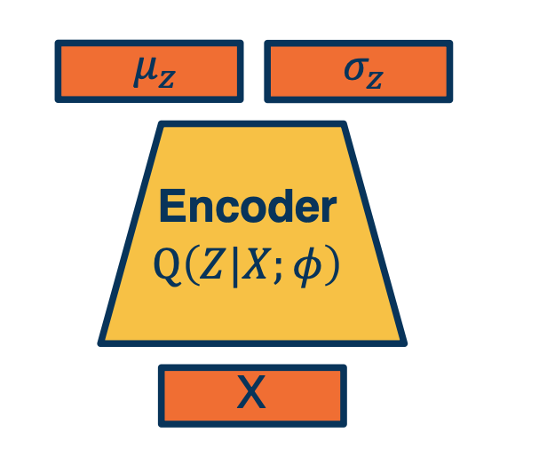
- Given an image, estimate $z$
- Again, output parameters of a distribution.
Given x, it will output not a particular $z$ but it will output the parameters of a Gaussian distribution $\mu$ and $\sigma$. If we want to generate an actual $z$ we can just sample from the parameters.
Putting it together
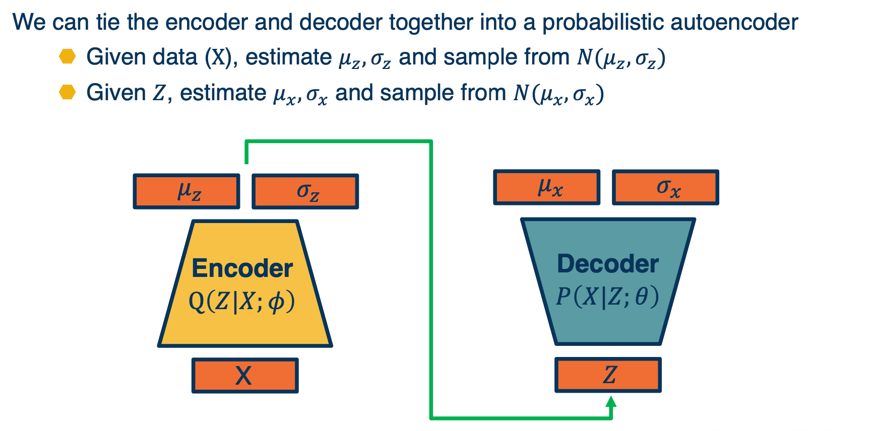
We can tie the encoder and decoder together into a probabilistic autoencoder
- Given data $X$, estimate $\mu_z, \sigma_z$ and sample from $N(\mu_z,\sigma_z)$
- Given $Z$, estimate $\mu_x,\sigma_x$ and sample from $N(\mu_x,\sigma_x)$
Maximizing likelihood
How can we optimize the parameters of the two networks?
Now equipped with our encoder and decoder networks, let’s work out the (log) data likelihood:
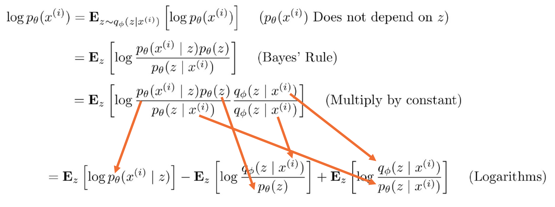
Recall that for KL-divergence (distance measure for distributions), always $\geq 0$,
\[KL(q(z) \lvert\lvert p(z\lvert x)) = \mathbf{E}[log q(z)] - \mathbf{E} [log p(z\lvert z)]\]Then the above equations can be re-written as:
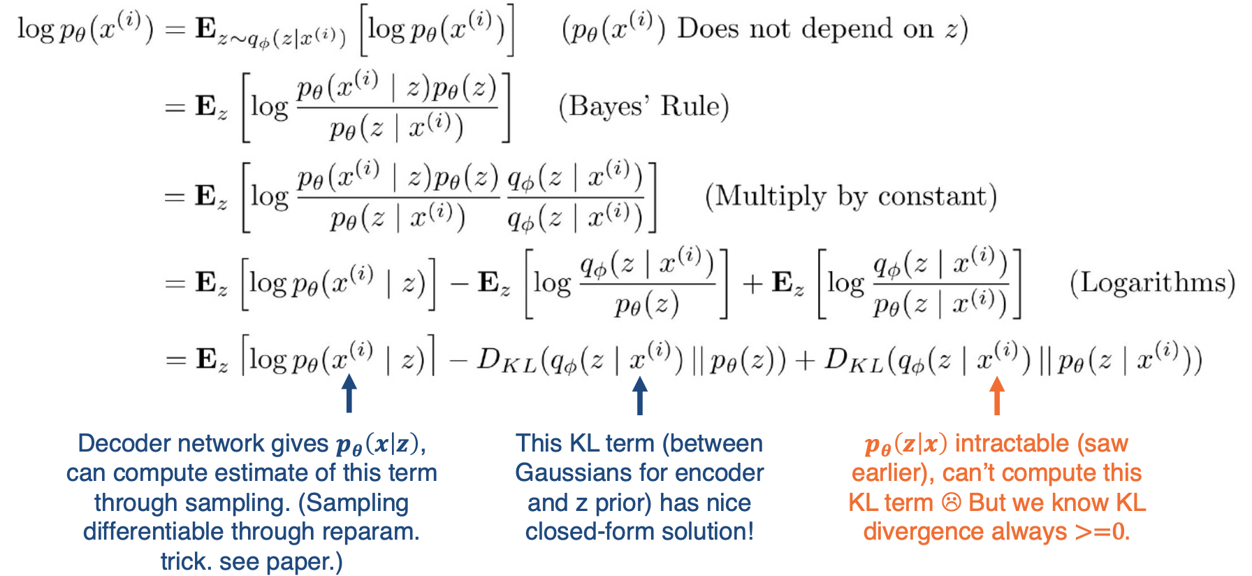
Note that the right hand side is actually intractable, so we are going to just ignore it. We know that KL divergence is always greater or equal to 0, and so if we just maximize the first two terms, we know that we will still be making progress.
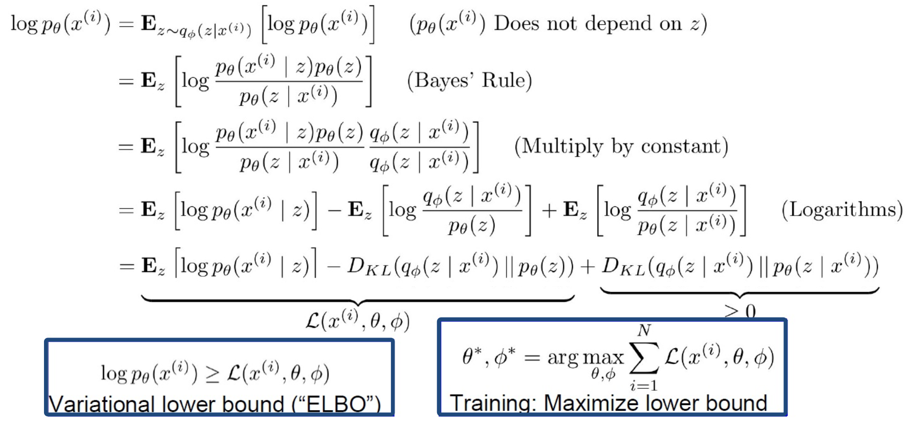
This is something called the variational lower bound or elbo, and it is actually a powerful technique that is used in many different places. The key idea is that if you are able to compute
Putting it together (again)
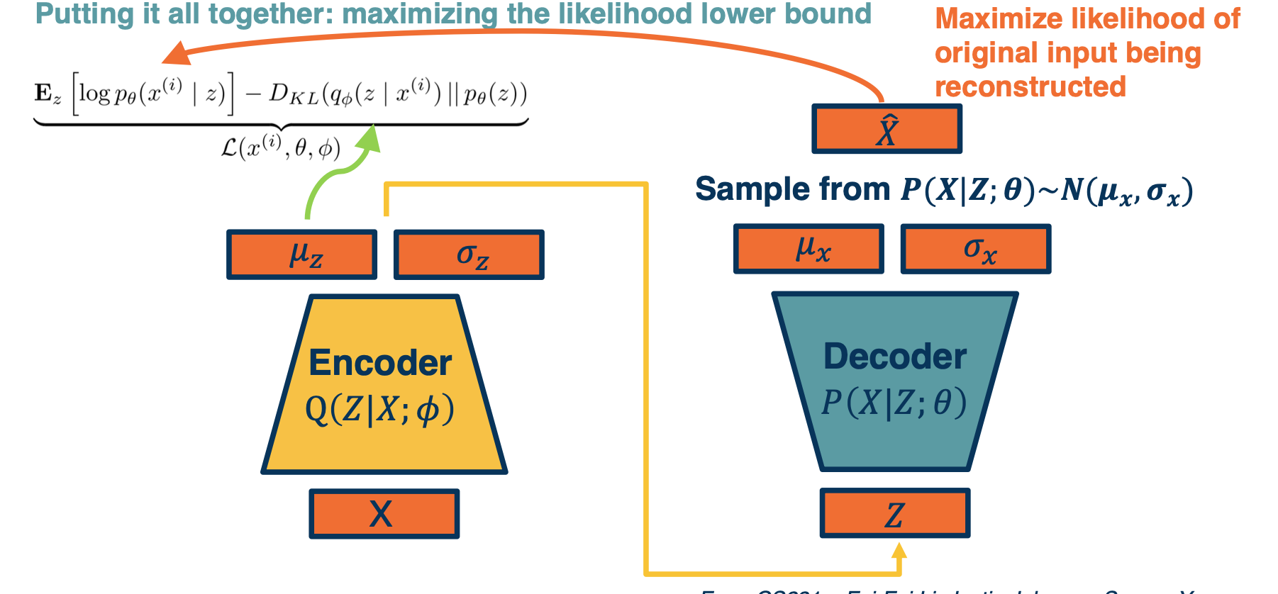
First, we will have a mini batch of unlabeled data x, and we will run it through our encoder $Q(Z \lvert X; \phi)$, this will be used to output parameters of a Gaussian distribution. This will be used to output parameters of a Gaussian distribution. Again, this is an assumption we make $\mu_z$ and $\sigma_z$. And so we’re going to make the approximate Posterior distribution close to the prior. That is we are going to take the KL divergence between $Q(Z\lvert X)$ , which is what we are computing here, and $P(z)$. Again this can be assumed to be a normal distribution, let’s say with a $\mu=0, \sigma=1$, and this is a KL divergence between two Gaussian distributions which actually can be computed in closed form.
We can then sample from this and generate a bunch of Z. And then we feed it through our decoder, which feeds it through $P(X\lvert Z;\theta)$ and generates $\mu_x,\sigma_x$. And now we can essentially maximize the likelihood of the original data being reconstructed. That is we are going to maximize the $log p(X\lvert Z)$, which is what our decoder is computing here.
However there are some problems, that can be addressed by reparameterization.
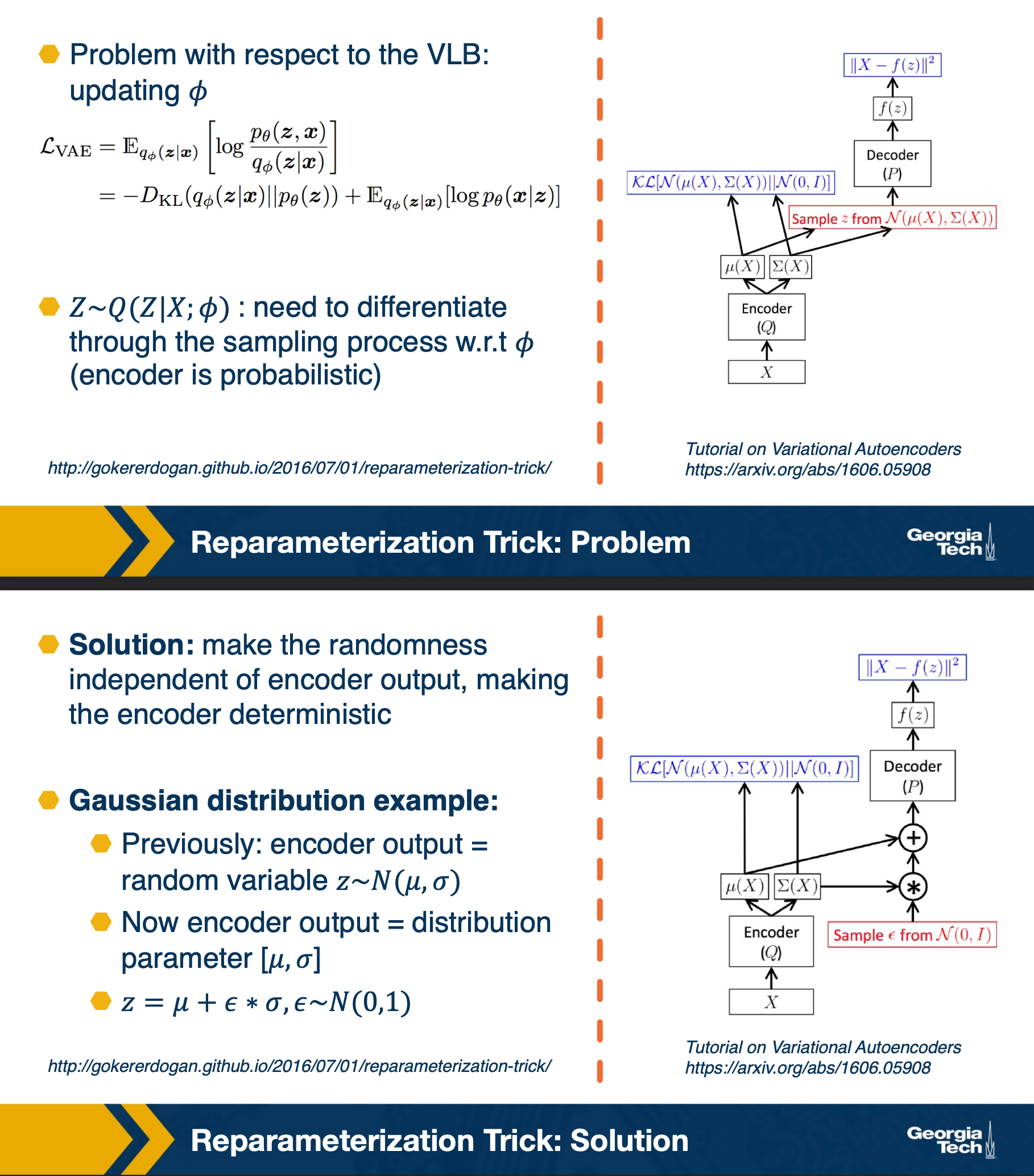
In summary,
Variational Autoencoders (VAEs) provide a principled way to perform approximate maximum likelihood optimization
- Requires some assumptions (e.g. Gaussian distributions)
Samples are often not as competitive as GANs
Latent features (learned in an unsupervised way!) often good for downstream tasks:
- Example: World models for reinforcement learning (Ha et al., 2018)