CS6515 OMSCS - Graduate Algorithms Notes

Posted Nov 11, 2024 Updated Dec 8, 2024

By yxlow

161 min read

Dynamic Programming

Introduction

Step1: State the subproblem, i.e define what $D[i][j][k]$ represents. In general:
- Try prefix (or suffix)
- Then try substrings
  - If you figured out a problem using substrings, think whether it can be solved with prefix/suffix.
  - At least for this course, we are not testing suffix.
Step2: Express the subproblem in the form of a recurrence relation, including the base cases.
Step3: Write out the pseudocode.
Step4: Time complexity analysis.

Longest increasing subsequence (LIS) (DP1)

Given a following sequence, find the length of the longest increasing subsequence. For example, given Input: 5, 7, 4, -3, 9, 1, 10, 4, 5, 8, 9, 3, the longest subsequence will be -3, 1, 4, 5, 8, 9, and the answer will be 6.

Extra Information:

When considering the LIS, the key question to ask is given a subsequence $x_1, …, x_{n-1}$, when will $x_n$ affect the LIS. When does this happen? Is only when $x_n$ is appended to the LIS of $x_1,…,x_{n-1}$.

Concretely, suppose the $LIS(x_1,…,x_{n-1}) = x_{1^*},…,x_j$, then LIS of $x_1,…,x_{n-1}, x_n$ will only change if $x_n$ is included, otherwise the LIS remains the same. This can only happen if $x_n > x_j$.

Subproblem:

Define the subproblem $L(i)$ to be be the length of the LIS on $x_1,…,x_i$. The important point is $L(i)$ must include $x_i$.

Recurrence relation:

\[L(i) = 1 +\underset{1 \leq j < i}{max} \{ L(j) \lvert x_j < x_i\ \}\]

Pseudocode:

Note, $L(i)$ must be at least 1, where the LIS is just itself.

S = [x1,...,xn]
L = [0, ..., 0]
for i = 1-> n:
  # Stores the current best of L[i], which must be at least 1
  L[i] = 1 
  for j = 1 -> i-1:
    if S[i] > S[j] and L[j] + 1 >= L[i]:
       L[i] = L[j] + 1 # Update current best

return max(L)

Complexity:

There is a double for loop with $i$ taking up to the value $n$. Hence, the time complexity is $O(n^2)$ and space complexity is $O(n)$.

Longest Common Subsequence (DP1)

Given two sequences, $x_1,..,x_n$ and $y_1,…,y_m$, find the longest common subsequence. For example given X = BCDBCDA and Y = ABECBAB, then the longest subsequence is BCBA.

Extra information:

Note that X and Y can be of different lengths, so, given a $X[:i]$ and $Y[:j]$. Let $L(i,j)$ denote the LCS of $X[:i]$ and $Y[:j]$, then there are two cases to consider:

if $x_i \neq y_j$, then either of the 3 cases can occur:

$x_i$ is not used in the final solution, $L(i-1,j)$
$y_j$ is not used in the final solution, $L(i, j-1)$
Both is not used in the final solution
- If the last character of both is not used, then we can just drop both!

So, we can just consider the first two cases and take the max, i.e max$(L(i-1,j), L(i,j-1))$

if $x_i = y_j$, again there are 3 cases to consider:

$x_i$ is not used in the final solution, $L(i-1,j)$
$y_i$ is not used in the final solution, $L(i, j-1)$
Both $x_i$ and $y_j$ are used in the final solution, $1+L(i-1,i-j)$.
- Note this means that the LCS $X[:i],Y[:j]$ ends with both $x_i$ and $y_j$ respectively

This is equal to max$\{L(i-1,j), L(i,j-1), 1+L(i-1,i-j)\}$.

However, we only need to consider the last case $1+L(i-1,i-j)$. This is because if the final solution must contain either $x_i$ or $y_j$ - otherwise we can just simply append them to the end. It may be possible that $x_i = y_{j-c}$, where it corresponds to some earlier occurrence in Y. But if this is true, that means $y_{j-c} = y_j$ and it does not matter.

Subproblem:

Let $L(i,j)$ denote the LCS of $X[:i],Y[:j]$, where $1 \leq i\leq n, 1\leq j \leq m$

Recurrence relation:

Firstly, $L(0,j) = 0, L(i,0) = 0$, then:

\[L(i,j) = \begin{cases} max(L(i-1,j), L(i,j-1)), & \text{if } x_i \neq y_j\\ 1+L(i-1,j-1), & \text{otherwise} \end{cases}\]

Pseudocode:

for i = 1->n:
  L[i][0] = 0
for j = 1->m:
  L[0][j] = 0
for i = 1->n:
  for j = 1->m:
     if X[i] == Y[j]:
       L[i][j] = 1+ L[i-1][j-1]
     else:
       L[i][j] = max(L[i-1][j], L[i][j-1])

return L[n][m]

Complexity:

Two loops, $n$ and $m$, so $O(nm)$

Backtracking

After the matrix L is constructed, we can backtrace to find out the common subsequence until we reach $L[1][1]$ - (note, this might be 0,0 depending on the indexing you use).

We consider the following cases:

If $x_i = y_j$, this means that a character was added and then we move diagonally up.
Else, we check to the left and top of coordinates (i,j).
- The left coordinate is (i-1,j)
- The top coordinate is (i,j-1)
- If the left coordinate is greater or equal to the top coordinate, we move left.
  - This means we ignored $x_i$
- Else, we move top.
  - This means that we ignored $y_j$
Repeat until converge to initial starting point.

i=n, j=m
string = ""
while i > 1 and j>1:
  if X[i] == Y[j]:
    string = string + X[i]
    i = i - 1
    j = j - 1
  if L[i-1][j] >= L[i][j-1]:
    i = i - 1
  else:
    j = j - 1  

return reverse(string)

Extra note - the steps of $i = i - 1$ and $j = j - 1$ can be reversed, and may lead to different results if there are multiple valid LCS.

Contiguous Subsequence Max Sum (DP1)

A contiguous subsequence of a list S is a subsequence made up of consecutive elements of S. For instance, if S is 5, 15, −30, 10, −5, 40, 10, then 15, −30, 10 is a contiguous subsequence but 5, 15, 40 is not. Give a linear-time algorithm for the following task:

Input: A list of numbers, a1, a2, . . . , an.

Output: The contiguous subsequence of maximum sum (a subsequence of length zero has sum zero).

For the preceding example, the answer would be 10, −5, 40, 10, with a sum of 55.

(Hint: For each j ∈ {1, 2, . . . , n}, consider contiguous subsequences ending exactly at position j.)

Extra notes:

Considering $S(i)$ which includes $x_i$. Since $x_i$ is part of the solution, then, the max sum is either itself, or add optimal max sum before itself if it is positive, i.e $S(i-1)$.

Subproblem:

Let $S(i)$ denote the max sum of the sequence $x_1,…,x_i$ including i.

Recurrence relation:

\[S(i) = a_i + max \{ 0, S(i-1) \}\]

Pseudocode:

seq = [s0,s1,...,sn]
S = [0,...,0]
for i -> 1 to n:
  S[i] = seq[i] + max(0,S[i-1])
return max(S)

Complexity:

Only one for loop, hence $O(n)$.

Knapsack (DP2)

Given $n$ items with weights $w_1,w_2,…, w_n$ each with value $v_1,…,v_n$ and capacity $W$, we want to find the subset of objects S, such that we maximize values max($\sum_{i\in S} v_i$ ) but $\sum_{i \in S} w_i < B$ where $B$ is the capacity of the bag.

Extra notes:

Problem 1:

Obviously, a greedy approach is bad, and the time complexity is $O(2^n)$, where each bit represents whether the object is included or not included.

Problem 2:

Consider the following problem, where we have 4 objects, with values 15,10,8,1 and weights 15,12,10,5 with total capacity 22. The optimal solution is items 2,3.

Then, K(1) = $x_1$ with $V=15$, K(2) is also $x_1$ with $V=15$. But, how do we express K(3) in terms of K(2) and K(1) which took the first object? So there is no real way to define K in terms of its previous sub problems!

Consider this new approach $K(I,B)$ where we also consider w as part of the sub problem - that is what is the optimal set of items given capacity b, for $ 1 \leq I \leq N, 1 \leq b \leq B$. Then by doing so, when we consider $K(3,22)$, there are two cases to consider:

If $x_3$ is part of the solution, then we look up $K(2,22-v_3) = K(2,12)$
- Notice that $K(2,12)$ will give us item 2 with $w_2 = 12$.
If $x_3$ is not part of the solution, then we look up $K(2,22)$

Subproblem:

Define $K(i,b)$ to be the optimal solution involving the first $i$ items with capacity $b$, $\forall i \in [1,N], w \in [1,B] $

Recurrence relation:

The recurrence can be defined as follows:

\[K(i,b) = max(v_i + K(i-1, b - w_i), K(i-1,b))\]

The base cases will be $K(0,b) = 0, K(i,0) = 0 \forall i, b$

That is, if item $x_i$ is included, then we add the corresponding value $v_i$ and subtract the weight of item i $w_i$. If it is not included, then we simply take the first $i-1$ items.

Pseudocode:

K = zeros(N,W)
weights = [w1,...,wn]
values = [v1,...,vn]
for i = 1 to N:
  K[i,0] = 0
for b = 1 to B:
  K[0, b] = 0
for i = 1 to N:
  for b = 1 to B:
    K[i,b] =  max(values[i] + K[i-1, b - w_i], K[i-1,b])

return K(N,W)

Complexity:

There is two loops, N, and W, so, $O(NB)$.

However, note that $B$ is an integer which can be represented with $2^m$ bits, so the complexity can be rewritten as $O(N2^m)$ which is exponential runtime.

Knapsack is also known as a Pseudo-polynomial time problem
Why is knapsack problem pseudo polynomial?

To do backtracking,

# Starting from index 1
included = [0] * N

for i = 1 to N:
  if K[i,b] != K[i-1,B]:
    # this means item i is included 
    included[i] = 1
    B = B - weights[i]

Then, included will be a binary representation of which items to be included.

Knapsack with repetitions (DP2)

This problem is a variant of the earlier problem, but you can add an infinite amount of $x_i$ in your knapsack.

Subproblem and Recurrence relation::

We can do the same as the above problem, and updating $K(i-1, b-w_i)$ to $K(i,b-w_i)$

\[K(i,b) = max(v_i + K(i, b-w_i), K(i-1,b))\]

But notice that this can be further simplified, we do not need to take into consideration of item $x_i$. We can just simply at each step, iterate through all the possible items to find the best item to add to the knapsack.

\[K(b) = \underset{i}{max} \{ v_i + K(w - w_i): i \leq i \leq n, w_i \leq b \}\]

Pseudocode:

for w = 1 to B:
  K(b) = 0
  for i = 1 to N:
    # if item x_i is below the weight limit and beats the current best
    if w_i <= w & K(b) < v_i + K(b-w_i):
      K(b) = v_i + K(b-w_i)
return K(B)

Complexity:

The complexity does not change, but the space complexity is now based on B.

Backtracking

To do backtracking, we have a separate array (multiset) $S(b) = [[],…,[]]$ so whenever an item $x_i$ get added, simply set $S(w) = S(w-w_i) + [i]$.

Note, if we find a better solution to add item $x_i$, then $S(w)$ will be overwritten.

Chain Multiply (DP2)

Consider two matrices $X_{a,b}$ and $Y_{b,c}$, the computation cost of calculating $XY$ is $O(abc)$.

Suppose we have 3 matrices $A_{2,5}, B_{5,10}, C_{10,2}$,

Calculating $((AB)C)$ will require $\underbrace{2 \times 5 \times 10}_{AB} + 2\times 10\times 2 = 140$ computations
While calculating $(A(BC))$ will require $\underbrace{5\times 10\times 2}_{BC} + 2\times 5\times 2 = 120$ computations

So, the point here is that the order of multiplication matters.

The problem now is given an initial sequence of matrices $A_1…,A_n$, suppose the optimal point to split is at $k$, then the left sequence will be $A_1….A_k$. Then, for this left sequence, what will be the optimal split? So, the point at which the split occurs is dynamic.


graph TD;

A --> B1
A --> B2

A["$$A_i A_{i+1}...A_j$$"]
B1["$$A_i ... A_l$$"]
B2["$$A_{l+1}... A_n$$"]

Remember, for a dynamic programming solution, each of the subtrees must also be optimal.

Subproblem:

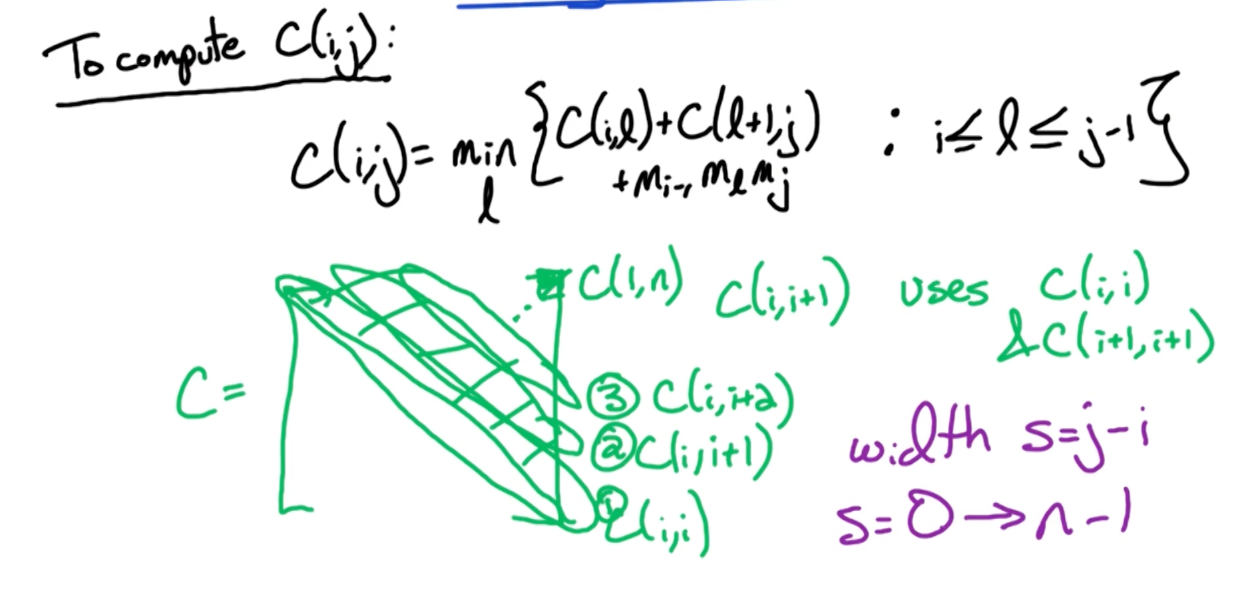
So, we denote $C(i,j)$ be the optimal cost of multiplying $A_i…A_j$

For an arbitrary matrix, $A_i$, the dimensions is $m_{i-1},m_{i}$

Recurrence relation:

\[C(i,j)=\underset{l}min\left\{ C(i,l)+C(l+1,j) +(m_{i-1} m_l m_j) \; i \le l \le j-1 \right\}\]

where $C(i,l)$ is the cost of the left subtree, $c(l+1,j)$ is the right substree and $m_{i-1} m_l m_j$ is the cost of combining the two sub trees.

Pseudocode:

So, $C(i,i) = 0, \forall i$. Then, we calculate $C(i,i+1), C(i, i+2), …, C(1,n)$ which is the solution that we are looking for.

Start at the diagonal and move up, to index this, consider $C(i,i+2)$ and $C(i,i)$, the difference is $i+2$, and $i$. Let’s call this the width, $s = j-i$.
- Then, $j$ can be calculated with $j = i+s$
- So we do this until we get width = $n-1$, so $s=0\rightarrow n-1$.

To rephrase this, given that we fill the diagonal first, we move one step to the right of the diagonal, i.e $C(2,i+1),.., C(n, i+1)$. Then, how many elements do we need to compute? n-1 elements.

Now, suppose we move $s$ steps to the right of the diagonal, then, there will be $n-s$ elements to compute.

# This step will populate the diagonals
for i=1 -> n:
  C(i,i)=0
# How many steps we move to the right of the diagonal
for s=1 -> n-1:
    # How many elements we need to compute
    for i=1 -> n-s:
      # Compute the j coordinate    
      Let j=i+s                                              
      C(i,j) = infinity
      for l=i -> j-1:                                          
        curr = (m[i-1] * m[l] * m[j]) + C(i,l) + C(l+1,j)
        if C(i,j) > curr:
          C(i,j) = curr
return C(1,n)

Complexity:

The time complexity is 3 inner for loops, so, $O(n^3)$.

Backtracking

To perform backtracking, we need another matrix, to keep track for each $i,j$, what is the corresponding $l$ in which the best split took place. Then, backtracking can be done via recursion. Here is an example:

def traceback_optimal_parens(s, i, j):
    if i == j:
        return f"A{i+1}"  # Single matrix, no parenthesis needed
    else:
        k = s[i][j]
        # Recursively find parenthesization for the left and right subchains
        left_part = traceback_optimal_parens(s, i, k)
        right_part = traceback_optimal_parens(s, k + 1, j)
        return f"({left_part} x {right_part})"

This divides each step into two subproblems, and the combine steps is a constant function, so, $T(n) = 2 T ( n/ 2) + 1$. Using master theorem, the time complexity is $O(n)$.

Extra notes on chain multiply:

  


# this is how far away from the diagonals
for width in range(1,n):
  """
  For example if you are 2 away from the diagonal,
  means you need n-2 x coordinates
  """
  for i in range(n - width):
    """
    This is the corresponding y coordinate,
    which is just adding the width to the x coordinate 
    From the current x-coordinate, move width steps.

    For example, lets look at the diagonal 2 points away

    (0,0), (0,1), (0,2), (0,3), (0,4)
    (_,_), (1,1), (1,2), (1,3), (1,4)
    (_,_), (_,_), (2,2), (2,3), (2,4)
    (_,_), (_,_), (_,_), (3,3), (3,4)
    (_,_), (_,_), (_,_), (_,_), (4,4)

    which is (0,2), (1,3), (2,4)
    so, x runs from 0 to 2 
    while y runs from 2 to 4 which is adding the width
    """
    j = i + width
    for l in range(i,j):
      """
      This l is the split, suppose i = 0, j = 5
      0|1234, 01|234, 012|34, 0123|4 which is considering
      all combinations
      """
      # D[i][j] = Operation(D[i][l],D[l+1][j])

Bellman-Ford (DP3)

Given $\overrightarrow{G}$ with edge weights and vertices, find the shortest path from source node $s$ to target node $z$. We assume that it has no negative weight cycles (for now).

Subproblem:

Denote $P$ to be the shortest path from $s$ to $z$. If there are multiple $P$ possible, we can assume any one of them. Since $P$ visits each vertex at most once, then:

\[\lvert P \lvert \leq (n-1)\text{edges}\]

DP idea: Condition on the prefix of the path. Use $i = 0 \rightarrow n-1$ edges on the paths.

For $0 \leq i \leq n-1, z \in V$, let $D(i,z)$ denote the length of the shortest path from S to Z using $\leq i$ edges.

Recurrence relation:

Base case: $D(0,s) = 0 \forall z \neq s, D(0, z) = \infty$

\[D(i,z) = \underset{y:\overrightarrow{yz}\in E}{min} \{D(i-1,y) + w(y,z), D(i-1,Z) \}\]

If there is no solution, then, it will still be $\infty$.

Otherwise, suppose the edge z is reachable from y, then there are two cases to consider. Consider the intermediate edge from y to z, if this edge $\overrightarrow{yz}$ is in the solution, add $w(y,z)$. The other case is a solution already exists without $\overrightarrow{yz}$, which will be denoted by $D(i-1,Z)$. We simply take the minimum of the two.

Pseudocode:

For z = 1 to length(V):
  D(0, z) = infinity
for i = 1 to n-1:
  for all z in V:
    D(i,z) = D(i-1,z)
      for all edges(y,z) in E:
        if D(i,z) > D(i-1,y) + w(y,z):
          D(i,z) = D(i-1,y) + w(y,z)
# Return the last row
Return D(n-1,:) 

Note, the last row basically returns all paths at most length $n-1$ from source node $s$ to all other vertex $z \in V$

Complexity:

Initially, you might think that there the complexity is $O(N^2E)$ because of the 3 nested for loops. But, in the 2nd and 3rd nested for loop, it is actually going through all edges (If you go through all nodes and all the edges within each node, it is actually going through all the edges). So the time complexity is actually $O(NE)$.

Now, how can you use bellman ford to detect if there is a negative cycle? Notice that the algorithm runs until n-1. Run it for one more time, and compare the difference. If the solution is different, then, some negative weights must exists.

In other words, check for:

\[D(n,z) < D(n-1,z), \exists z \in V\]

Suppose we wanted to find all pairs, and use bellman ford, what will the solution look like?

Given $\overrightarrow{G} = (V,E)$, with edge weights $w(e)$. For $y,z \in V$, let $dist(y,z)$ be the legnth of shortest path $y \rightarrow z$..

Goal: Find $dist(y,z), \forall y,z \in V$

The time complexity in this case will be $O(N^2M)$. Also, if $\overrightarrow{G}$ is a fully connected graph, it means there are $M=N^2$ edges, making it a $O(N^4)$ algorithm. What can we do about this? Look at Flord Warshall!

A side note about Dijkstra algorithm, it is a greedy algorithm with time complexity $O(N + E log(N))$, so it is better than Bellman Ford if you know that there are no negative edges

Floyd-Warshall (DP3)

Subproblem:

For $0 \leq i \leq n$ and $1 \leq s, t \leq n$, let $D(i,s,t)$ be the length of the shortest path from $s\rightarrow t$ using a subset ${1, …, i}$ as intermediate vertices. Note, the key here is intermediate vertices.

So, $D(0,s,t)$ means you can go to t from s directly without any intermediate vertices.

Recurrence relation:

The base case is when $i = 0$, then there are two cases, either you can go to t from s, in which case it is $w_{s,t}$, else $\infty$.

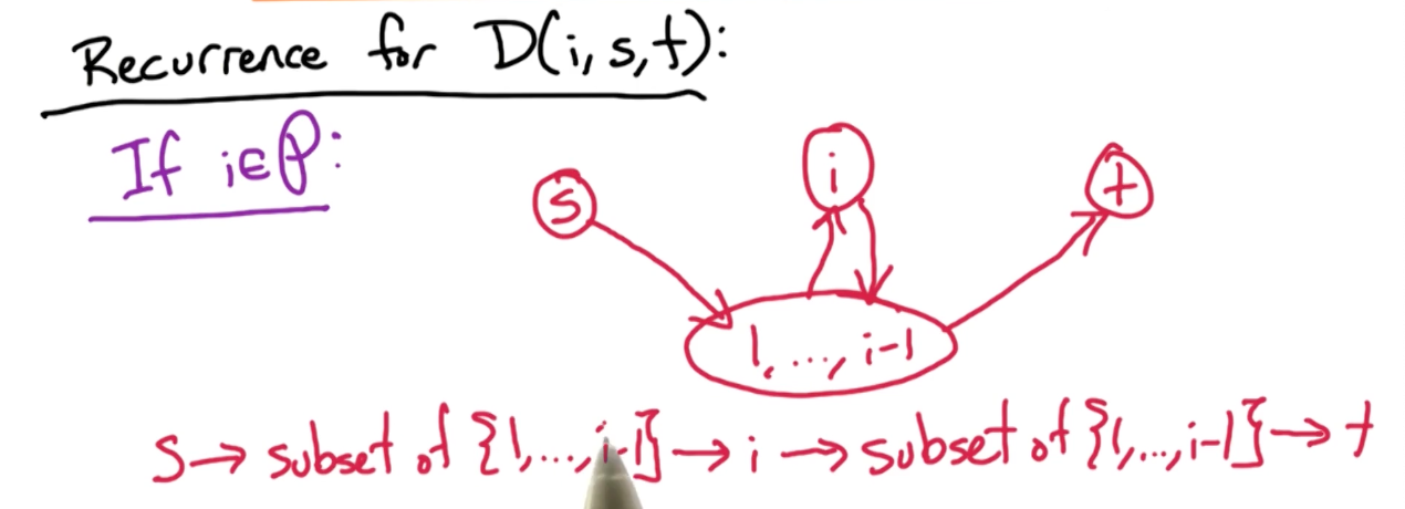
What about $D(i,s,t)$? There are again two cases to consider, either the intermediate vertex $i$ is in the path $P$ or otherwise.

If it is not in the optimal path $P$, then the $D(i,s,t) = D(i-1,s,t)$.

If it is in the optimal path $P$, then this is the scenario where it can happen.

Notice that you go from $S$ to a subset (can be an empty set) or vertices ${1,…,i-1}$, go to vertex $i$, back to the subset before reaching vertex $t$. So there is this 4 paths to consider.

So, the first two paths can be represented by $D(i-1, s,i)$, that is using the subset of vertices ${1,…,n-1}$ to reach vertex $i$, and, the next two paths can be represented by $D(i-1,i,t)$, that is reaching vertex $t$ from $i$ using subset of vertices ${1,…,n-1}$

Pseudocode:

Inputs: G, w

for s=1->n:
    for t=1->n:
        if (s,t) in E 
            then D(0,s,t)=w(s,t)
        else D(0,s,t) = infty

for i=1->n:
    for s=1->n:
        for t=1->n:
            D(i,s,t)=min{ D(i-1,s,t), D(i-1,s,i) + D(i-1,i,t) }

# return the last slice, has N^2 entries.
Return D(n,:,:)

Complexity:

The complexity here is clearly $O(N^3)$.

To detect negative weight cycles, can check the diagonal of the matrix D.

If there is a negative cycle, then there should be a negative path length from a vertex to itself, i.e $D(n,y,y) < 0, \exists y \in V $.
- This is equivalent to checking whether there is any negative entries on the diagonal matrix $D(n,:,:)$.

For bellman ford algorithm, it depends on the s and z to determine if a negative weight path exists, a single source shortest path algorithm. But for Floyd Warshall, it does all pair shortest path, and hence it is guaranteed to find the negative cycle, if it exists.

Divide and conquer

Master theorem

Note, this is the simplified form of the Master Theorem, which states that:

\[T(n) = \begin{cases} O(n^d), & \text{if } d > \log_b a \\ O(n^d \log n), & \text{if } d = \log_b a \\ O(n^{\log_b a}), & \text{if } d < \log_b a \end{cases}\]

For constants $a>0, b>1, d \geq 0$.

The recurrence relation under the Master Theorem is of the form:

\[T(n) = aT\left(\frac{n}{b}\right) + O(n^d)\]

where:

$a$: Number of subproblems the problem is divided into.
$b$: Factor by which the problem size is reduced.
$O(n^d)$: Cost of work done outside the recursive calls, such as dividing the problem and combining results.

Understanding the Recursion Tree

To analyze the total work, think of the recursion as a tree where:

Each level of the tree represents a step in the recursion.
The root of the tree represents the original problem of size $n$.
The first level of the tree corresponds to dividing the problem into $a$ subproblems, each of size $\frac{n}{b}$.
The next level corresponds to further dividing these subproblems, and so on.

Cost at the $k-th$ level:

Number of Subproblems:
\[\text{Number of subproblems at level } k = a^k\]
At each split, it produces $a$ sub problems, after $k$ splits, hence $a^k$.
Size of Each Subproblem:
\[\text{Size of each subproblem at level } k = \frac{n}{b^k}\]
During each step, the problem is reduced by $b$. E.g in binary search, each step reduces by half, $\frac{n}{2}$. After $k$ steps, it will be $\frac{n}{2^k}$
Cost of Work at Each Subproblem:
\[\text{Cost of work at each subproblem at level } k = O\left(\left(\frac{n}{b^k}\right)^d\right)\]
This is the cost of merging. For example in merge sort, cost of merging is $O(n)$ which is linear.
Thus, total cost at level k :
\[\text{Total cost at level } k = a^k \times O\left(\left(\frac{n}{b^k}\right)^d\right) = O(n^d) \times \left(\frac{a}{b^d}\right)^k\]

Then, $k$ goes from $0$ (the root) to $log_n b$ levels (leaves), so,

\[\begin{aligned} S &= \sum_{k=0}^{log_b n} O(n^d) \times \left(\frac{a}{b^d}\right)^k \\ &= O(n^d) \times \sum_{k=0}^{log_b n} \left(\frac{a}{b^d}\right)^k \end{aligned}\]

Recall that for geometric series, $\sum_{i=0}^{n-1} ar^i = a\frac{1-r^n}{1-r}$. So, we need to consider $\frac{a}{b^d}$. So, when $n$ is large:

Case 1:

If $d> log_b a$, then $ a < b^d $ thus $\frac{a}{b^d} < 1$. So when $n$ is large,

\[\begin{aligned} S &= O(n^d) \times \sum_k^\infty (\frac{a}{b^d})^k \\ &= O(n^d) \times \frac{1}{1-\frac{a}{b}} \\ &\approx O(n^d) \end{aligned}\]

For case 1, the work is dominated by the cost of the non-recursive work (i.e., the work done in splitting, merging, or processing the problem outside of the recursion) dominates the overall complexity.

Case 2:

if $d = log_b a$, then $a = b^d$ thus $\frac{a}{b^d} = 1$.

\[\begin{aligned} S &= O(n^d) \times \sum_k^{log_b n} \underbrace{(\frac{a}{b^d})^k}_{1} \\ &= O(n^d) \times log_b n \\ &\approx O(n^d log_b n) \\ &\approx O(n^d log n) \\ \end{aligned}\]

Notice that the log base is just a ratio that we can further simplify.

For case 2, The work is evenly balanced between dividing/combining the problem and solving the subproblems. Another way to think about it is, at each step there is $n^d$ work, with $log_b n \approx log n $ levels, so the total work is $O(n^d log n)$

Case 3:

If $d < log_b a$ then $a > b^d$ thus $\frac{a}{b^d} > 1$.

\[\begin{aligned} S &= O(n^d) \times \sum_{k=0}^{log_b n} (\frac{a}{b^d})^k \\ &= O(n^d) \times \frac{(\frac{a}{b^d})^{log_b n}-1}{\frac{a}{b^d}-1}\\ &\approx O(n^d) \times (\frac{a}{b^d})^{log_b n}-O(n^d) \\ &\approx O(n^d) \times (\frac{a}{b^d})^{log_b n}\\ &= O(n^d) \times \frac{a^{log_b n}}{(b^{log_b n})^d}\\ &= O(n^d) \times \frac{a^{log_b n}}{n^d}\\ &= O(a^{log_b n}) \\ &= O(a^{(log_a n)(log_b a)}) \\ &= O(n^{log_b a}) \end{aligned}\]

For case 3, the work is dominated by the cost of recursive subproblems dominates the overall complexity

Fast Integer multiplication (DC1)

Given two (large) n-bit integers $x \& y$, compute $ z = xy$.

Recall that we want to look at the running time as a function of the number of bits. The naive way will take $O(N^2)$ time.

Inspiration:

Gauss’s idea: multiplication is expensive, but adding/subtracting is cheap.

2 complex numbers, $a+bi\ \&\ c+di$, wish to compute $(a+bi)(c+di) = ac - bd + (bc + ad)i$. Notice that in this case we need 4 real number multiplications, $ac,bd,bc,ad$. Can we reduce this 4 multiplications to 3? Can we do better?

Obviously it is possible! The key is that we are able to compute $bc+ad$ without computing the individual terms; not going to compute $bc, ad$ but instead $bc+ad$, consider the following:

\[\begin{aligned} (a+b)(c+d) &= ac + bd + (bc + ad) \\ (bc+ad) &= \underbrace{(a+b)(c+d)}_{term3} - \underbrace{ac}_{term1} - \underbrace{bd}_{term2} \end{aligned}\]

So, we need to compute $ac, bd, (a+b)(c+d)$ to obtain $(a+bi)(c+di)$. We are going to use this idea to multiply the n-bit integers faster than $O(n^2)$

Input: n-bits integers x,y and assume $n$ is a power of 2 - for easy computation and analysis.

Idea: break input into 2 halves of size $\frac{n}{2}$, e.g $x = x_{left} \lvert x_{right}$, $y = y_{left} \lvert y_{right}$

Suppose $x=2=(10110110)_2$:

$x_{left} = x_L = (1011)_2 = 11$
$x_{right} = x_R= (0110)_2 = 6$
Note, $182 = 11 \times 2^4 + 6$
In general, $x = x_L \times 2^{\frac{n}{2}} + x_R$

Divide and conquer:

\[\begin{aligned} xy &= ( x_L \times 2^{\frac{n}{2}} + x_R)( y_L \times 2^{\frac{n}{2}} + y_R) \\ &= 2^n \underbrace{x_L y_L}_a + 2^{\frac{n}{2}}(\underbrace{x_Ly_R}_c + \underbrace{x_Ry_L}_d) + \underbrace{x_Ry_R}_b \end{aligned}\]

EasyMultiply(x,y):
input: n-bit integers, x & y , n = 2**k
output: z = xy 
xl = first n/2 bits of x, xr = last n/2 bits of x
same for yl, yr.

A = EasyMultiply(xl,yl), B= EasyMultiply(xr,yr)
C = EasyMultiply(xl,yr), D= EasyMultiply(xr,yl)

Z = (2**n)* A + 2**(n/2) * (C+D) + B
return(Z)

running time:

$O(n)$ to break up into two $\frac{n}{2}$ bits, $x_L,x_R, y_L,y_R$
To calculate A,B,C,D, its $4T(\frac{n}{2})$
To calculate $z$, is $O(n)$
- Because e.g we need to shift $A$ by $2^n$ bits.

So the total complexity is: $4T(\frac{n}{2}) + O(n)$

Let $T(n)$ = worst-case running time of EasyMultiply on input of size n, and by master theorem, this yields $O(n^{log_2 4}) = O(n^2)$

As usual, as with everything, can we do better? Can we change the number 4 to something better like 3? I.e we are trying to reduce the number of 4 sub problems to 3.

Better approach:

\[\begin{aligned} xy &= ( x_L \times 2^{\frac{n}{2}} + x_R)( y_L \times 2^{\frac{n}{2}} + y_R) \\ &= 2^n \underbrace{x_L y_L}_1 + 2^{\frac{n}{2}}(\underbrace{x_Ly_R + x_Ry_L}_{\text{Change this!}}) + \underbrace{x_Ry_R}_4 \end{aligned}\]

Using Gauss idea:

\[\begin{aligned} (x_L+x_R)(y_L+y_R) &= x_L y_L + x_Ry_R + (x_Ly_R+x_Ry_L) \\ (x_Ly_R+x_Ry_L) &= \underbrace{(x_L+x_R)(y_L+y_R)}_{c}- \underbrace{x_L y_L}_a + \underbrace{x_Ry_R}_b \\ \therefore xy &= 2^n A + 2^{\frac{n}{2}} (C-A-B) + B \end{aligned}\]

FastMultiply(x,y):
input: n-bit integers, x & y , n = 2**k
output: z = xy 
xl = first n/2 bits of x, xr = last n/2 bits of x
same for yl, yr.

A = FastMultiply(xl,yl), B= FastMultiply(xr,yr)
C = FastMultiply(xl+xr,yl+yr)

Z = (2**n)* A + 2**(n/2) * (C-A-B) + B
return(Z)

With Master theorem, $3T(\frac{n}{2}) + O(n) \rightarrow O(n^{log_2 3})$

Example:

Consider $z=xy$, where $x=182, y=154$.

$x = 182 = (10110110)_2, y= 154 = (10011010)_2$
- $x_L = (1011)_2 = 11$
- $x_R = (0110)_2 = 6$
- $y_L = (1001)_2 = 9$
- $y_R = (1010)_2 = 10$
$A = x_Ly_L= 11*9 = 99$
$B = x_Ry_R = 6*10 = 60$
$C = (x_L + x_R)(y_L + y_R) = (11+6)(9+10) = 323 $

\[\begin{aligned} z & = 2^n A + 2^{\frac{n}{2}} (C-A-B) + B\\ &= 2^8* 99 + 2^4 * (323-99-60) + 60 \\ &= 28028 \end{aligned}\]

Linear-time median (DC2)

Given an unsorted list $A=[a_1,…,a_n]$ of n numbers, find the median ($\lceil \frac{n}{2}\rceil$ smallest element).

Quicksort Recap:

Choose a pivot p
Partition A into $A_{< p}, A_{=p}, A_{>p}$
Recursively sort $A_{< p}, A_{>p}$

Recall in quicksort the challenging component is choosing the pivot, and if we reduce the partition by only 1, this results in the worse case can result in $O(n^2)$. So what is a good pivot? the median but how can we find this median without sorting which is $O(n log n)$.

The key insight here is we do not need to consider all of $A_{< p},A_{=p}, A_{>p}$, we just need to consider 1 of them.

Select(A,k):
Choose a pivot p (How?)
Partition A in A < p, A = p, A > p          
if  k <= |A_{<p}|        
    then return Select(A_{<p},k)               
if  |A_{<p}| < k <= |A_{>p}| + |A_{=p}|           
    then return p            
if  k > |A_{>p}| + |A_{=p}|  
    then return Select(A_{>p}, k - |A_{<p}| - |A_{=p})| 

The question becomes, how do we find such a pivot?

The pivot matters a lot, because if the pivot is the median, then, our partition will be $\frac{n}{2}$ which fields $T(n) = T(\frac{n}{2}) + O(n)$, which will achieve a running time of $O(n)$.

However, it turns out we do not need $\frac{1}{2}$, we just need something that can reduce the problem at each step, for example $T(n) = T(\frac{3n}{4}) + O(n)$ where each step only eliminates $\frac{1}{4}$ of the problem space, which will still give us $O(n)$. It turns out we just need the constant factor to be less than 1 (do you know why?), so, even 0.99 will work!

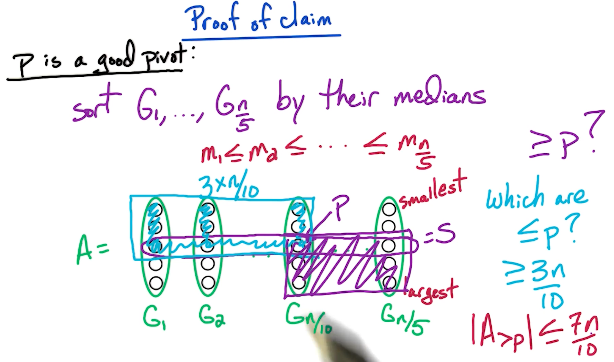
For the purpose of this lectures, we consider a pivot $p$ is good, if it reduces the problem space by $\frac{1}{4}$. i.e $\lvert A_{<p} \lvert \leq \frac{3n}{4} \& \lvert A_{>p} \lvert \leq \frac{3n}{4} $.

Assume for now we have a sorted array, then, the probability of selecting a good pivot is when the number is between $[\frac{n}{4},\frac{3n}{4} ]$, so the probability is half. We can validate the pivot by tracking the size of the split. So this is as good as flipping a coin - what is the expected number of trails before you get a heads? The answer is 2. However, there is still a chance that you keep getting tails, so it does not still guarantee the worst case runtime is $O(n)$. Consider the following:

\[\begin{aligned} T(n) &= T\bigg(\frac{3}{4} n\bigg) + \underbrace{T\bigg(\frac{n}{5}\bigg)}_{\text{cost of finding good pivot}} + O(n)\\ &\approx O(n) \end{aligned}\]

To accomplish this, choose a subset $S \subset A$, where $\lvert S \rvert = \frac{n}{5}$. Then, we set the pivot = $median(S)$.

But, now we face another problem, how do we select this sample $S$? - one problem after another.

Introducing FastSelect(A,k):

Input:   A - an unsorted array of size n
         k an integer with 1 <= k <= n 
Output:  k'th smallest element of A

FastSelect(A,k):

Break A into ceil(n/5) groups         G_1,G_2,...,G_n/5
    # doesn't matter how you break A

For j=1->n/5:
    sort(G_i)
    let m_i = median(G_i)

S = {m_1,m_2,...,m_n/5}             # these are the medians of each group
p = FastSelect(S,n/10)              # p is the median of the medians (= median of elements in S)
Partition A into A_<p, A_=p, A_>p

# now recurse on one of the sets depending on the size
# this is the equivalent of the quicksort algorithm 

if k <= |A_<p|:
    then return FastSelect(A_<p,k)    
if k > |A_>p| + |A_=p|:
    then return FastSelect(A_>p,k-|A_<p|-|A_=p|)
else return p

Analysis of run time:

Splitting into $\frac{n}{5}$ groups - $O(n)$
Since we are sorting a fix number of elements (5), it is order $O(1)$, over $\frac{n}{5}$, so, it is still $O(n)$.
The first FastSelect takes $T(\frac{n}{5})$ time.
The final recurse takes $T(\frac{3n}{4})$

\[\begin{aligned} T(n) &= T(\frac{3n}{4})+ T(\frac{n}{5}) + O(n) \\ &= O(n) \end{aligned}\]

The key here is $\frac{3}{4} + \frac{1}{5} < 1$

Prove of the claim that p is a good pivot

Fun exercise: Why did we choose size 5? And not size 3 or 7?

Recall earlier, for blocks of 5, the time complexity is given by:

\[T(n) = T(\frac{n}{5}) + T(\frac{7n}{10}) + O(n)\]

and, $\frac{7}{10} + \frac{1}{5} < 1$.

Now, let us look at the case of 3, assuming we split into n/3 groups:

21  ... n/6 1 ... n/3 1
22  ... n/6 2 ... n/3 2
23  ... n/6 3 ... n/3 3 

Number of elements: 2 * n/6 = n/3. Likewise, our remaining partition is of size 2n/3.

Then our formula will look:

\[\begin{aligned} T(n) &= T(\frac{2n}{3})+ T(\frac{n}{3}) + O(n) \\ &= O(n logn) \end{aligned}\]

Similarly, suppose we use size 7,

Number of elements less than or equal to n/14 4 is n/14 * 4 = 2n/7.
Number of remaining elements more than n/14 4 is 5n/7.

In this case, we get the equation:

\[\begin{aligned} T(n) &= T(\frac{5n}{7})+ T(\frac{n}{7}) + O(n) \\ &= O(n) \end{aligned}\]

Although in this case we still achieve $O(n)$, even though $\frac{5}{7} + \frac{1}{7} = 0.85 < \frac{1}{5} + \frac{7}{10} = 0.9$, we increased the cost of sorting our sub list sorting. (Nothing is free! )

For more information, feel free to look at this link by brillant.org!

Solving Recurrences (DC3)

Merge sort: $T(n) = 2T(\frac{n}{2}) + O(n) = O(nlogn)$
Naive Integer multiplication: $T(n) = 4T(\frac{n}{2}) + O(n) = O(n^2)$
Fast Integer multiplication: $T(n) = 3T(\frac{n}{2}) + O(n) = O(n^{log_2 3})$
Median: $T(n) = T(\frac{3n}{4}) + O(n) = O(n)$

An example:

For some constant $c>0$, and given $T(n) = 4T(\frac{n}{2}) + O(n)$:

\[\begin{aligned} T(n) &= 4T(\frac{n}{2}) + O(n) \\ &\leq cn + 4T(\frac{n}{2}) \\ &\leq cn + 4[T(4\frac{n}{2^2} + c \frac{n}{2})]\\ &= cn(1+\frac{4}{2}) + 4^2 T(\frac{n}{2^2}) \\ &\leq cn(1+\frac{4}{2}) + 4^2 [4T\frac{n}{2^3} + c(\frac{n}{2^2})] \\ &= cn (1+\frac{4}{2} + (\frac{4}{2})^2) + 4^3 T(\frac{n}{2^3}) \\ &\leq cn(1+\frac{4}{2} + (\frac{4}{2})^2 + ... + (\frac{4}{2})^{i-1}) + 4^iT(\frac{4}{2^i}) \end{aligned}\]

If we let $i=log_2 n$, then $\frac{n}{2^i}$ = 1.

\[\begin{aligned} &\leq \underbrace{cn}_{O(n)} \underbrace{(1+\frac{4}{2} + (\frac{4}{2})^2 + ... + (\frac{4}{2})^{log_2 n -1})}_{O(\frac{4}{2}^{log_2 n}) = O(n^2/n) = O(n)} + \underbrace{4^{log_2 n}}_{O(n^2)} \underbrace{T(1)}_{c}\\ &= O(n) \times O(n) + O(n^2) \\ &= O(n^2) \end{aligned}\]

Geometric series

\[\begin{aligned} \sum_{j=0}^k \alpha^j &= 1 + \alpha + ... + \alpha^k \\ &= \begin{cases} O(\alpha^k), & \text{if } \alpha > 1 \\ O(k), & \text{if } \alpha = 1 \\ O(1), & \text{if } \alpha < 1 \end{cases} \end{aligned}\]

The first case is what happened in Naive Integer multiplication
The second case is the merge step in merge sort, where all terms are the same.
The last step is finding the median where $\alpha = \frac{3}{4}$

Manipulating polynomials

It is clear that $4^{log_2 n} = n^2$, what about $3^{log_2 n} = n^c$

First, note that $3 = 2^{log_2 3}$

\[\begin{aligned} 3^{log_2n} &= (2^{log_2 3})^{log_2 n} \\ &= 2^{\{log_2 3\} \times \{log_2 n\}} \\ &= (2^{log_2 n})^{log_2 3} \\ &= n^{log_2 3} \end{aligned}\]

Another example: $T(n) = 3T(\frac{n}{2}) + O(n)$

\[\begin{aligned} T(n) &\leq cn(1+\frac{3}{2} + (\frac{3}{2})^2 + ... + (\frac{3}{2})^{i-1}) + 3^iT(\frac{3}{2^i}) \\ &\leq \underbrace{cn}_{O(n)} \underbrace{(1+\frac{3}{2} + (\frac{3}{2})^2 + ... + (\frac{3}{2})^{log_2 n -1})}_{O(\frac{3}{2}^{log_2 n}) = O(3^{log_2 n}/2^{log_2 n})} + \underbrace{3^{log_2 n}}_{3^{log_2 n}} \underbrace{T(1)}_{c}\\ &= \cancel{O(n)}\times O(3^{log_2 n}/\cancel{2^{log_2 n}}) + O(3^{log_2 n}) \\ &= O(3^{log_2 n}) \end{aligned}\]

General Recurrence

For constants a > 0, b > 1, and given: $T(n) = a T(\frac{n}{b}) + O(n)$,

\[T(n) = \begin{cases} O(n^{log_b a}), & \text{if } a > b \\ O(n log n), & \text{if } a = b \\ O(n), & \text{if } a < b \end{cases}\]

Feel free to read up more about master theorem!

FFT (DC4+5)

FFT stands for FAst Fourier Transform.

Polynomial Multiplication:

\[\begin{aligned} A(x) &= a_0 + a_1x + a_2 x^2 + ... + a_{n-1} x^{n-1} \\ B(x) &= b_0 + b_1x + b_2 x^2 + ... + b_{n-1} x^{n-1} \\ \end{aligned}\]

We want:

\[\begin{aligned} C(x) &= A(x)B(x) \\ &= c_0 + c_1x + c_2 x^2 + ... + c_{2n-2} x^{2n-2} \\ \text{where } c_k &= a_0 b_k + a_1 b_{k-1} + ... + a_kb_0 \end{aligned}\]

We want to solve, given $a = (a_0, a_1, …, a_{n-1}), b= (b_0, b_!, …, b_{n-1})$, compute $c = a*b = (c_0, c_1, …, c_{2n-2})$

Note, this operation is called the convolution denoted by *.

For the naive algorithm, it will take $O(k)$ time for $c_k, \rightarrow O(n^2)$ total time. We are going to introduce a $O(nlogn)$ time algorithm.

Polynomial basics

Two Natural representations for $A(x) = a_0 + a_1 x + … + a_{n-1}x^{n-1}$
- coefficients $a = (a_0, …, a_{n-1})$
  - More intuitive to represent
- values: $A(x_1), …, A(x_n)$
  - Easier to use to multiply

Lemma: Polynomial of degree $n-1$ is uniquely determine by its values at any $n$ distinct points.

For example, a line is determined by two points, and, in general a $n-1$ polynomial is defined by any $n$ points on that polynomial.

What FFT does, is it $values \Longleftrightarrow coefficients$

Take coefficients as inputs
Convert to values
Multiply,
Convert back

One important point is that FFT converts from the coefficients to the values, not for any choice of $x_1,…,x_n$ but for a particular well chosen set of points. Part of the beauty of the FFT algorithm is this choice.

MP: values

Key idea: Why is it better to multiply in values?

Given $A(x_1), … ,A(x_{2n}), B(x_1), …, B(X_2n)$, we can compute

\[C(x_i) = A(x_i)B(x_i), \forall 1 \geq x \geq 2n\]

Since each step is O(1), the total running time is $O(n)$. We will show that the conversion to values using FFT is $O(nlogn)$ while the values step is $O(n)$. Note, why do we take A and B at two n points? Well, C is a polynomial of degree at most 2n-2, so we needed at least $2n-1$ points, so $2n$ suffices.

FFT: opposites

Given $a = (a_0, a_1,…, a_{n-1})$ for poly $A(x) = a_0 + a_1x+…+a_{n-1}x^{n-1}$, we want to compute $A(x_1), …., A(x_{2n})$

The key thing to note that we get to choose the 2n points $x_1,…,x_{2n}$.
- How to choose them?
The crucial observation is suppose $x_1,…,x_n$ are opposite of $x_{n+1},…,x_{2n}$
- $x_{n+1} = -x_1, …, x_{2n} = -x_n$
- Suppose our $2n$ points satisfies this $\pm$ property
- We will see how this property will be useful.

FFT: splitting $A(x)$

Look at $A(x_i) \& A(x_{n+i} = A(-x_i))$, lets break these up to even and odd terms.

Even terms are of the form $a_{2k}x^{2k}$
- Since the powers are even, this is the same for $A(x_i) = A(x_{n+i})$.
Odd terms are $a_{2k+1}x^{2k+1}$
- Then these are the opposite, $A(-x_i) = A(x_{n+i})$.

(Note, this was super confusing for me, but, just read on)

So, it makes sense to split up $A(x)$ into odd and even terms. So, lets partition the coefficients for the polynomial into:

$a_{even} = (a_0, a_2, …, a_{n-2})$
$a_{odd} = (a_1, a_3, …, a_{n-1})$

FFT: Even and Odd

Again, given $A(x)= a_0 + a_1 x + … + a_{n-1}x^{n-1}$,

\[\begin{aligned} A_{even}(y) &= a_0 + a_2y + a_4y^2 + ... + a_{n-2}y^{\frac{n-2}{2}} \\ A_{odd}(y) &= a_1 + a_3y + a_5y^2 + ... + a_{n-1}y^{\frac{n-2}{2}} \\ \end{aligned}\]

Notice that both have degree $\frac{n}{2}-1$. Then, (take some time to convince yourself)

\[A(x) = A_{even} (x^2) + x A_{odd}(x^2)\]

Can you see the divide and conquer solution? We start with a $n$ size polynomial, and split it to two $\frac{n}{2}, A_{even},A_{odd}$

We reduce the original polynomial from size $n-1$ to $\frac{n-2}{2}$.
However, if we need a $x$ at two endpoints, we still need $A_{even}, A_{odd}$ endpoints the squared of these original two endpoints.
- So while the degree went down by a factor of two, but the number of points we need to evaluate has not gone down
- This is when we will make use of the $\pm$ property.

FFT: Recursion

Let’s suppose that the two end points that we want to evaluate satisfies the $\pm$ property: $x_1,…,x_n$ are opposite of $x_{n+1},…, x_{2n}$

\[\begin{aligned} A(x_i) &= A_{even}(x_i^2) + x_i A_{odd}(x_i^2) \\ A(x_{n+i}) &= \underbrace{A(-x_i)}_{opposite} = A_{even}(x_i^2) - x_i A_{odd}(x_i^2) \end{aligned}\]

Notice that the values are reused for $A_{even}(x_i^2), A_{odd}(x_i^2)$

Given $A_{even}(y_1), …, A_{even}(y_n) \& A_{odd}(y_1), …, A_{odd}(y_n)$ for $y_1 = x_1^2, …m y_n=x_n^2$, in $O(n)$ time get $A(x_1),…,A(x_2n)$.

FFT: summary

To get $A(x)$ of degree $\leq n-1$ at $2n$ points $x_1,…,x_{2n}$

Define $A_{even}(y), A_{odd}(y)$ of degree $\leq \frac{n}{2}-1$
Recursively evaluate at n points, $y_1 = x_1^2 = x_{n+1}^2, …, y_n = x_n^2 = x_{2n}^2$
In $O(n)$ time, get $A(x)$ at $x_1,…,x_{2n}$.

This gives us a recursion of

\[T(n) = 2T(\frac{n}{2}) + O(n) = O(nlogn)\]

FFT: Problem

Note that we need to choose numbers such that $x_{n+i} = -x_i$ for $i \in [1,n]$.

then the points we are considering are the square of these two end points $y_1 = x_1^2, …, y_n = x_n^2$, and we also want these end points to also satisfies the $\pm$ property.

But, what happens at the next level?

$y_1 = - y_{\frac{n}{2}+1}, …, y_{\frac{n}{2}} = -y_n$
So, we need $x_1^2 = - x^2_{\frac{n}{2}+1}$
- Wait a minute, but how can a positive number $x_1^2$ be equals to a negative number?
- This is where complex number comes in.

To be honest, I am super confused, I ended up watching this youtube video:

Complex numbers

Given a complex number $z = a+bi$ in the complex plane, or the polar coordinates $(r,\theta)$. Note that for some operations such as multiplication, polar coordinates is more efficient.

How to convert between complex plane and polar coordinates?

\[(a,b) = (r cos\theta, r sin\theta)\]

$r = \sqrt{a^2 + b^2}$
$\theta$ is a little more complicated, it depends which quadrant of the complex plane you are at.

There is also Euler’s formula:

\[re^{i\theta} = r(cos\theta + isin\theta)\]

So, multiplying in polar makes it really easy:

\[r_1e^{i\theta_1}r_2e^{i\theta_2} = (r1r2)e^{i(\theta_1 + \theta_2)}\]

complex roots

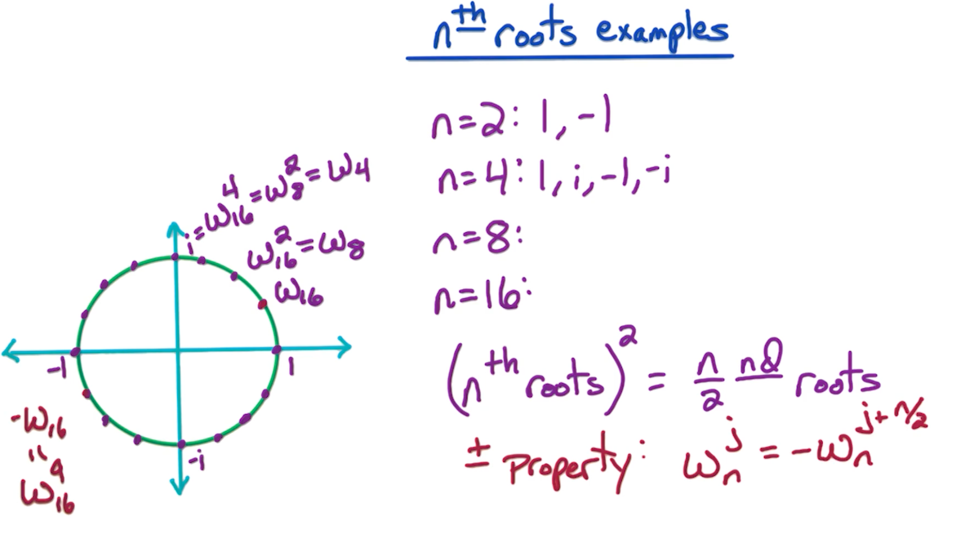
When n=2, roots are 1, -1
When n=4, roots are 1, -1, i, -i

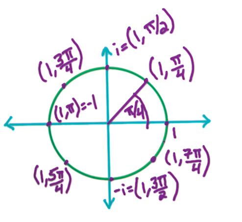
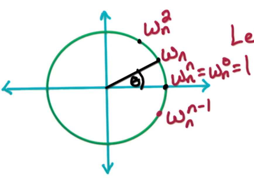
In general, the n-th roots of unity $z$ where $z^n = 1$ is $(1, 2\pi j)$ for integer $j$. $2\pi j$ is on the positive real axis, as $2\pi$ is one “loop” around the circle.

Note, since $r =1, r^n=1$ so they basically form a circle with radius 1 from the origin. Then,

\[n\theta = 2\pi j \Rightarrow \theta \frac{2\pi j}{n}\]

So the $n^{th}$ roots notation can be expressed as

\[(1, \frac{2\pi}{n}j), j \in [0,...,n-1]\]

We re-write this as:

\[\omega_n = (1, \frac{2\pi}{n}) = e^{2\pi i /n }\]

With that, we can formally define the the $n^{th}$ roots of unity, $\omega_n^0, \omega_n^1, …., \omega_n^{n-1}$.

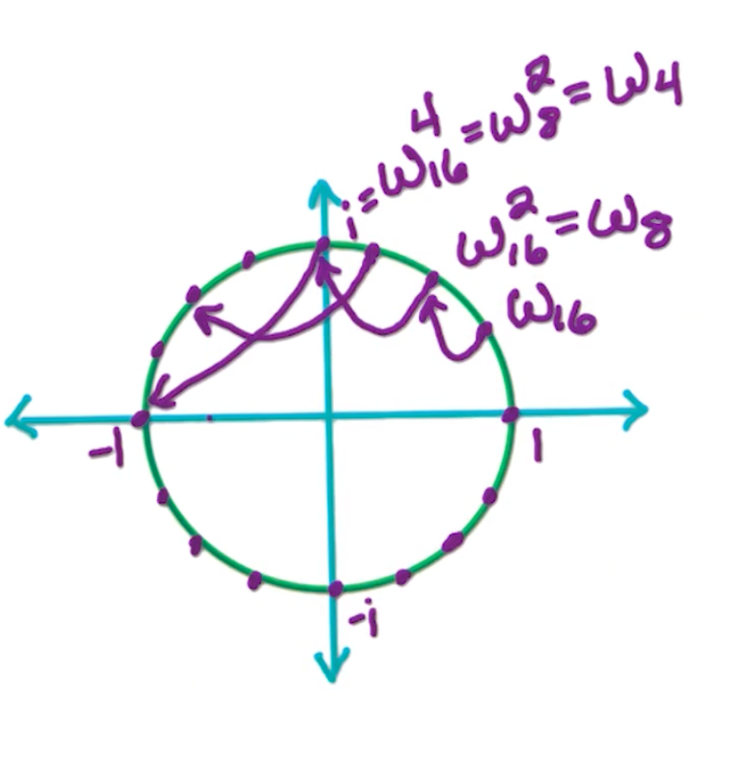
\[\omega_n^j = e^{2\pi ij /n } = (1, \frac{2\pi j}{n})\]

Suppose we want 16 roots, we can see the circle being divided into 16 different parts.

And, note the consequences:

$(n^{th} roots)^2 = \frac{n}{2} roots$
- e.g $\omega_{16}^2 = \omega_8$
Also, the $\pm$ property, where $\omega_{16}^1 = -\omega_{16}^9$

key properties

The first property - For even $n$, satisfy the $\pm$ property
- first $\frac{n}{2}$ are opposite of last $\frac{n}{2}$
- $\omega_n^0 = -\omega_n^{n/2}$
- $\omega_n^1 = -\omega_n^{n/2+1}$
- $…$
- $\omega_n^{n/2 -1} = -\omega_n^{n/2 + n/2 - 1} = -\omega_n^{n-1}$
The second property, for $n=2^k$,
- $(n^{th} roots)^2 = \frac{n}{2} roots$
- $(\omega_n^j)^2 = (1, \frac{2\pi}{n} j)^2 = (1, \frac{2\pi}{n/2} j) = w_{n/2}^j$
- $(\omega_n^{n/2 +j})^2 = (\omega_n^j)^2 = w_{n/2}^j $

So why do we need this property that the nth root squared are the n/2nd roots? Well, we’re going to take this polynomial A(x), and we want to evaluate it at the nth roots. Now these nth roots satisfy the $\pm$ property, so we can do a divide and conquer approach.

But then, what do we need? We need to evaluate $A_{even}$ and $A_{odd}$ at the square of these nth roots, which will be the $\frac{n}{2}$ nd roots. So this subproblem is of the exact same form as the original problem. In order to evaluate A(x) at the nth roots, we need to evaluate these two subproblems, $A_{even}$ and $A_{odd}$ at the $\frac{n}{2}$ nd roots. And then we can recursively continue this algorithm.

FFT Core

Again, the inputs are $a= (a_0, a_1, …, a_{n-1})$ for Polynomial $A(x)$ where n is a power of 2 with $\omega$ is a $n^{th}$ roots of unity. The desired output is $A(\omega^0), A(\omega^1), …, A(\omega^{n-1})$

We let $\omega = \omega_n = (1, \frac{2\pi}{n}) = e^{2\pi i/n}$

And the outline of FFT as follows:

if $n=1$, return $A(1)$
let $a_{even} = (a_0, a_2, …, a_{n-2}), a_{odd} = (a_1, …, a_{n-1})$
Call $FFT(a_{even},\omega^2)$ get $A_{even}(\omega^0), A_{even}(\omega^2) , …, A_{even}(\omega^{n-2})$
Call $FFT(a_{odd},\omega^2)$ get $A_{odd}(\omega^0), A_{odd}(\omega^2) , …, A_{odd}(\omega^{n-2})$
Recall that if $\omega = \omega_n$, then $(\omega^j_n)^2 = \omega_{n/2}^j$
- In other words, the square of n roots of unity gives us $n/2$ roots of unity.
For $j = 0 \rightarrow \frac{n}{2} -1$:
- $A(\omega^j) = A_{even}(\omega^{2j}) + \omega^j A_{odd}(\omega^{2j})$
- $A(\omega^{\frac{n}{2}+j}) = A(-\omega^j) = A_{even}(\omega^{2j}) - \omega^j A_{odd}(\omega^{2j})$
Return $(A(\omega^0), A(\omega^1), …, A(\omega^{n-1}))$

We can write this in a more concise manner:

if $n=1$, return $(a_0)$
let $a_{even} = (a_0, a_2, …, a_{n-2}), a_{odd} = (a_1, …, a_{n-1})$
Call $FFT(a_{even},\omega^2) = (s_0, s_1, …, s_{\frac{n}{2}-1})$
Call $FFT(a_{odd},\omega^2) = (t_0, t_1, …, t_{\frac{n}{2}-1})$
For $j = 0 \rightarrow \frac{n}{2} -1$:
- $r_j = s_j + w^j t_j$
- $r_{\frac{n}{2}+j} = s_j - w^j t_j$

The running time is given by the recurrence $2T(n/2) + O(n) = O(n log n)$

Inverse FFT view

We first express the forward direction:

For point $x_j$, $A(x_j) = a_0 + a_1x_j + a_2x_j^2 + , … + a_{n-1}x_j^{n-1}$

For points $x_0, x_1, …, x_{n-1}$:

\[\begin{bmatrix} A(x_0) \\ A(x_1) \\ \vdots \\ A(x_{n-1}) \end{bmatrix} = \begin{bmatrix} 1 & x_0 & x_0^2 & ... & x_0^{n-1} \\ 1 & x_1 & x_1^2 & ... & x_1^{n-1} \\ & & \ddots & & \\ 1 & x_{n-1} & x_{n-1}^2 & ... & x_{n-1}^{n-1} \\ \end{bmatrix} \begin{bmatrix} a_0 \\ a_1\\ \vdots \\ a_{n-1} \end{bmatrix}\]

We let $x_j = w_n^j$: (Note anything to power 0 is 1)

\[\begin{bmatrix} A(1) \\ A(\omega_n) \\ A(\omega_n^2)\\ \vdots \\ A(\omega_n^{n-1}) \end{bmatrix} = \begin{bmatrix} 1 & 1 & 1 & ... & 1 \\ 1 & \omega_n & \omega_n^2 & ... & \omega_n^{n-1} \\ 1 & \omega_n^2 & \omega_n^4 & ... & \omega_n^{2(n-1)} \\ & & \ddots & & \\ 1 & \omega_n^{n-1} & \omega_n^{2(n-1)} & ... & \omega_n^{(n-1)(n-1)} \\ \end{bmatrix} \begin{bmatrix} a_0 \\ a_1 \\ a_2 \\ \vdots \\ a_{n-1} \end{bmatrix}\]

Two interesting properties:

The matrix is symmetric
The matrix is made up of functions of $\omega_n$

We denote the above as

\[A = M_n(\omega_n) * a = FFT(a, \omega_n)\]

And the inverse can be calculated as:

\[M_n(\omega_n)^{-1} A = a\]

Without proof, it turns out that $M_n(\omega_n)^-1 = \frac{1}{n}M_n(\omega_n^{-1})$ (Feel free eto watch yourself)

What is $\omega_n^{-1}$ ? i..e $\omega_n \times \omega_n^{-1} = 1$

The inverse turns out to be $\omega_n^{n-1}$, $\omega_n \times \omega_n^{n-1} = \omega_n^n = \omega_n^0 = 1$

So,

\[M_n(\omega_n)^-1 = \frac{1}{n}M_n(\omega_n^{-1}) = \frac{1}{n}M_n(\omega_n^{n-1})\]

We did all this, so, the inverse FFT given $A$,is simply:

\[na = M_n(\omega_n^{n-1}) A = FFT(A, \omega_n^{n-1}) \\ \therefore a = \frac{1}{n} FFT(A, \omega_n^{n-1})\]

Poly mult using FFT

Input: Coefficients $a = (a_0, …, a_{n-1})$ and $b = (b_0, …, b_{n-1})$ Output: $C(x) = A(x)B(x)$ where $c = (c_0, …, c_{2n-2})$

FFT$(a,\omega_{2n}) = (r_0, …, r_{2n-1})$
FFT$(b,\omega_{2n}) = (s_0, …, s_{2n-1})$
for $j = 0 \rightarrow 2n-1$
- $t_j = r_j \times s_j$
Have $C(x)$ at $2n^{th}$ roots of unity and run inverse FFT
- $(c_0, …, c_{2n-1}) = \frac{1}{2n}FFT(t, \omega_{2n}^{2n-1})$

Graphs

Strongly Connected Components (GR1)

Here is a recap on DFS (for a undirected graph)

DFS(G):
  input G=(V,E) in adjacency list representation
  output: vertices labeled by connected components
  cc = 0
  for all v in V, visited(v) = False, prev(v) = NULL
  for all v in V:
    if not visited(v):
      cc++
      Explore(v)

Now lets define Explore:

Explore(z):
  ccnum(z) = cc
  visited(z) = True
  for all (z,w) in E:
    if not visited(w):
      Explore(w)
      prev(w) = z

The ccnum is the connected component number of $z$.

The overall running time is $O(n+m), n = \lvert V \lvert, m = \lvert M \lvert$. This is because you visit each node once, and, at each node, you try the edges, hence the total run time is total nodes and total edges in order to reach all nodes.

What if our graph is now directed? We can still use DFS, but add pre or postorder numbers and remove the counters.

Notice hte difference nad adding of the clock variable:

DFS(G):
  clock = 1
  for all v in V, visited(v) = False, prev(v) = NULL
  for all v in V:
    if not visited(v):
      cc++
      Explore(v)

Now lets define Explore:

Explore(z):
  pre(z) = clock;clock++
  visited(z) = True
  for all (z,w) in E:
    if not visited(w):
      Explore(w)
      prev(w) = z
  post(z) = clock; clock++

Here is an example:

Assuming we start at B, this is how our DFS looks like define as Node(pre,post):

Blue edge reflects that it is “used” during DFS but not used because the node has been visited.

There are various type of edges, for a given edge $z \rightarrow w$:

Treeedge such as $B\rightarrow A, A\rightarrow D$
- where $post(z) > post(w)$, because of how you recurse back up during DFS
Back edges $E \rightarrow A, F\rightarrow B$
- $post(z) < post(w)$
- Edges that goes back up.
Forward edges $D \rightarrow G, B \rightarrow E$
- Same as the tree edges
- $post(z) > post(w)$
Cross edges $F \rightarrow H, H \rightarrow G$
- $post(z) > post(w)$

Notice that only for the back edges it is different in terms of the post order and behaves differently from the other edges.

Cycles

A graph $G$ has a cycle if and only if its DFS tree has a back edge.

Proof:

Given $a \rightarrow b \rightarrow c \rightarrow … \rightarrow j \rightarrow a$ which is a cycle. Suppose somewhere down the line we have this node $i$, then the sub tree (descendants) of $i$ must contain $i-1$ which contains a backedge to $i$.

For the other direction, it is obvious, Consider the back edge $B \rightarrow A$, then the cycle exists.

Toplogical sorting

Topologically sorting a DAG (directed acyclic graph that has no cycles): order vertices so that all edges go from lower $\rightarrow$ higher. Recall that since it has no cycles, it has no back edges. So the post order numbers must be $post(z) > post(w)$ for any edge $z \rightarrow w$.

So, to do this, we can order vertices by decreasing post order number. Note that for this case, since we have $n$ vertices, we can create a array of size $2n$ and insert the nodes according to their post order number. So, our sorting of post order numbers runtime is $O(n)$.

What are the valid Topological order? : $XY(ZWU\lvert ZUW\lvert UZW)$

Note, for instance, XYUWZ is not a valid topological order! (Basically Z must come before W) - Because there’s a directed edge from Z to W, Z must come before W in any valid topological ordering of this graph.

Analogy: Imagine you’re assembling a toy. Piece Y is needed for both piece Z and piece W. But, piece Z is also needed for piece W. You must attach Y to Z first, then Z to W. Even though Y is needed for W, you don’t attach it directly to W.

DAG Structure

Source vertex: no incoming edges
- Highest post order
Sink vertex = no outgoing edges
- Lowest post order

By now, you are probably thinking, what does all this has to do with strongly connected component (SCC)? We will show that it is possible to do so with two DFS search.

Connectivity in DAG

Vertices $v$ & $w$ are strongly connected if there is a path $v \rightarrow w$ and $w \rightarrow v$

So, SCC defined as strongly connected component, is the maximal set of strongly connected vertices.

Example:

How many strongly connected components (SCC) does the graph has? 5

A is a SCC by itself since it can reach many other nodes but no other nodes can reach A
{H,I,J,K,L} Can reach each other
{C,F,G}
{B,E}
{D}

We can simplify the above graph to the following meta graph:

Notice that this meta graph is a DAG and it is always the case. This should be obvious because if two strongly connected components are involved in a cycle, then they will be combined to form a bigger SCC.

So, every directed graph is a DAG of it’s strongly connected components. You can take any graph, break it up into SCC and then topologically sort this SCC so that all edges go left to right.

Motivation

There are many ways we can do this, such as start with sinking vertices or source vertices. But, instead we can find the sink SCC, so, we find SCC S, output it, and remove it and repeat it. It turns out, Sinks SCC are easier to work with!

Recall we take any $v \in S$, where $S$ is the sick SCC. For example from the earlier graph we run Explore(v), and we run explore from any of of the vertices in {H,I,J,K,L}, we will explore these vertices and not any other because it is a sink SCC.

What if we find a vertex in the source component? You ended up exploring the whole graph, too bad! So, how can we be smart about this and find a vertex that lies in a sink component? Because if we can do so (somehow magically select a vertex in the sink SCC), then we are guaranteed to find all the nodes in the sink SCC.

So, how can we find such a vertex?

Recall that in a DAG, the vertex with the lowest postorder number is a sink.

In a directed directed G, can we use the same property? Does the property for a general graph, such that v with the lowest post order always lie in a sink SCC? HA of course its not true, do you think it will be that easy?

Notice that B has the lowest post order (3) but it belongs to the SCC {A,B}.

What about the other way around? Does v with the highest post order always lie in a source SCC? Turns out, this is true! How can we make use of this? Simple, just reverse it! So the source SCC of the reverse graph is the sink SCC!

So, for directed $G=(V,E)$, look at $G^R = (V,E^R)$, so, the source SCC in $G$ = sink SCC in $G^R$. So, we just flip the graph, run DFS, take the highest post order which is the source SCC in $G^R$, that will be the sink in $G$.

Example of SCC

lets consider the same graph but now we reverse it, and we start at node C

We start from c from the reverse graph $G^R$, find the SCC at {C, G, F, B, A, E}, then we proceed to {D} before going to {L}. you may notice that the choosing of which vertex might be important, suppose you pick at any vertex at {H,I,J,K,L}, it will be able to reach all vertices except {D} so that starting vertex will still have the highest post number.

Then, we sort it and get this following order: L, K, J, I, H, D, C, B, E, A, G, F. So now, we run DFS from the original graph starting at $G$.

At first step, we start at $L$, so, we will reach {L,K,J,I,H} label as 1 and strike them out.
We then visit $D$, and reach {D}, label as 2 and strike them out
We do the same for $C$, reach {C,F,G} label as 3 and strike them out
Then do the same for {B,E} label as 4
and finally {A} label as 5

So, the L, K, J, I, H, D, C, B, E, A, G, F is mapped to {1,1,1,1,1,2,3,4,4,5,3,3}. Another interesting observation of the new labels {1,2,3,4,5} , we have the following graph:

Notice that this metagraph, they go from $5 \rightarrow to 1$. So, the {1,1,1,1,1,2,3,4,4,5,3,3} also outputs the topological order in reverse order! So we can take any graph, run two iterations of DFS, finds its SCC, and structure these SCC in topological order.

SCC algorithm

SCC(G):
  input: directed G=(V,E) in adjacency list
  1. Construct G^R
  2. Run DFS on G^R
  3. Order V by decreasing post order number
  4. Run undirected connected components alg on G based on the post order number

Proof of claim:

Given two SCC $S$ and $S’$, and there is an edge $v \in S \rightarrow w \in S’$, the claim is the max post number in $S$ is always greater than max post number of $S’$.

The first case is if we start from $z \in S’$, then, we finish exploring in $S’$ before moving to $S$, so post numbers in $S$ will be bigger.

The second case is if we start $z \in S$, then $z$ will be the root node since we can travel to $S’$ from $z$. Since $z$ is the root node, then it must have the highest post order number.

BFS & Dijkstras

DFS : connectivity

BFS:

input: $G=(V,E)$ & $s \in V$

output: for all $v \in V$, dist(v) = min number of edges from $s$ to $v$ and $prev(v)$.

Dijkstra’s:

input: $G=(V,E)$ & $s \in V$, $\ell(e) > 0 \forall e \in E$

output: $\forall v \in V$, dist(v) = length of shortest $s\rightarrow v$ path.

Note, Dijkstra uses the min-heap (known as priority queue) that takes $logn$ insertion run time. So, the overall runtime for Dijkstra is $O((n+m)logn)$.

2-Satisfiability (GR2)

Boolean formula:

$n$ variables with $x_1, …, x_n$
$2n$ literals $x_1, \bar{x_1}, …, x_n, \bar{x_n}$ where $\bar{x_i} = \lnot x_i$
We use $\land$ for the and condition and $\lor$ for the or condition.

CNF

Now, we define CNF (conjunctive normal form):

Clause: OR of several literals $(x_3 \lor \bar{x_t} \lor \bar{x_1} \lor x_2)$ F in CNF: AND of m clauses: $(x_2) \land (\bar{x_3} \lor x_4) \land (x_3 \lor \bar{x_t} \lor \bar{x_1} \lor x_2) \land (\bar{x_2} \lor \bar{x_1})$

Notice that for F to be true, that means for each condition we need at least one literal to be true.

SAT

Input: formula f in CNF with $n$ variables and $m$ clauses

output: assignment (assign T or F to each variable) satisfying if one exists, NO if none exists.

Example: $ f = (\bar{x_1} \lor \bar{x_2} \lor x_3) \land (x_3 \lor x_3) \land (\bar{x_3} \lor \bar{x_1}) \land (\bar{x_3})$

And an example that will work is $x_1 = F, x_2 = T, x_3 = F$.

K-SAT

For K sat, the input is formula f in CNF with $n$ variables and $m$ clauses each of size $\leq k$. So the above function $f$ is an example. In general:

SAT is NP-complete
K-SAT is NP complete $\forall k \geq 3$
Poly-time algorithm using SCC for 2-SAT

For example consider the following input f for 2-SAT:

\[f = (x_3 \lor \bar{x_2}) \land (\bar{x_1}) \land (x_1 \lor x_4) \land (\bar{x_4} \lor x_2) \land (\bar{x_3} \lor x_4)\]

We want to simplify unit-clause which is a clause with 1 literal such as $(\bar{x_1})$. This is because to satisfy $\bar{x_1}$ there is only one way to set $x_1 = F$.

Take a unit clause say literal $a_i$
Satisfy it (set $a_i = T$)
Remove clauses containing $a_i$ and drop $\bar{a_i}$
let $f’$ be the resulting formula

For example:

\[\begin{aligned} f &= (x_3 \lor \bar{x_2}) \land (\cancel{\bar{x_1}}) \land (\cancel{x_1} \lor x_4) \land (\bar{x_4} \lor x_2) \land (\bar{x_3} \lor x_4) \\ &= (x_3 \lor \bar{x_2}) \land (x_4) \land (\bar{x_4} \lor x_2) \land (\bar{x_3} \lor x_4) \end{aligned}\]

So, the original $f$ is satisfiable if $f’$ is. Notice that there is a unit clause $(x_4)$ and we can remove it. Eventually I am either going to left with an empty set, or a formula where all clauses are of size 2.

SAT-graph

Take $f$ with all clauses of size $=2$, $n$ variables and $m$ clauses, we create a directed graph:

$2n$ vertices corresponding to $x_1, \bar{x_1}, …, x_n, \bar{x_n}$
$2m$ edges corresponding to 2 “implications” per clause

Consider the following example: $f = (\bar{x_1} \lor \bar{x_2}) \land (x_2 \lor x_3) \land (\bar{x_3} \lor \bar{x_1})$

Notice that if we set $x_1 = T \rightarrow x_2 = F$, and likewise $x_2 = T \rightarrow x_1 = F$

In general given $(\alpha \lor \beta)$, then you need $\bar{\alpha} \rightarrow \beta$ and $\bar{\beta} \rightarrow \alpha$

If we observe the graph, we notice that there is a path from $x_1 \rightarrow \bar{x_1}$, which is a contradiction. If $x_1 = F$, then it might be ok? In general, if there are paths such that $x_1 \rightarrow \bar{x_1}$ and $\bar{x_1} \rightarrow x_1$, then $f$ is not satisfiable because $\bar{x_1},x_1$ is in the same SCC.

In general:

If for some $i$, $x_i, \bar{x_i}$ are in the same SCC, then $f$ is not satisfiable.
If for some $i$, $x_i, \bar{x_i}$ are in different SCC, then $f$ is satisfiable.

2-SAT Algo

Take source scc $S’$ and set $S’ = F$
Take sink scc $\bar{S’}$ and set $\bar{S’} = T$
When we done this, then we can remove all these literals from the graph!

This works because of a key fact: if $\forall i$, $x_i \bar{x_i}$ are in different SCC’s, then $S$ is a sink SCC if and only if $\bar{S}$ is a source SCC.

2SAT(F):
  1. Construct graph G for f
  2. Take a sink SCC S 
    - Set S = T ( and bar(S) = F)
    - remove S, bar(S)
    - repeat until empty

Proof:

The first claim is we show that path $\alpha \to \beta \iff \bar{\beta} \to \bar{\alpha}$

Take path $\alpha \to \beta$, say $\gamma_0 \to \gamma_1 \to … \to \gamma_l$ where $\gamma_0 = \alpha, \gamma_l = \beta$

Recall that $(\bar{\gamma_1} \lor \gamma_2)$ is represented in the graph as $(\gamma_1 \to \gamma_2)$, since if $\gamma_1 = T$ then $\gamma_2$ must also be $T$. $(\bar{\gamma_1} \lor \gamma_2)$ is also represented in the graph as $(\bar{\gamma_2} \to \bar{\gamma_1})$. This shows that $\bar{\gamma_0} \gets \bar{\gamma_1} \gets … \gets \bar{\gamma_l}$ which implies $\bar{\beta} \to \bar{\alpha}$ since $\gamma_0 = \alpha, \gamma_l = \beta$.

Using this claim, we can show 2 more things:

If $\alpha,\beta \in S$, then $\bar{\alpha}, \bar{\beta} \in \bar{S}$. This is true because if there are paths in $\alpha \leftrightarrow \beta$ since they are in the same SCC, this means that there are paths $\bar{\beta} \leftrightarrow \bar{\alpha}$ using the above claim and they belong to SCC.

It remains to show that $S$ must be a sink SCC and $\bar{S}$ is a source SCC.

We take a sink SCC S, for $\alpha \in S$, that means there are no edges from $\alpha \to \beta$ which implies no edges such that $\bar{\beta} \to \bar{\alpha}$. In other words, no outgoing edges from $\alpha$ means there is no incoming edges to $\bar{\alpha}$. This shows that $\bar{S}$ is a source SCC!

MST (GR3)

For the minimum spanning tree, we are going to go through the krusal algorithm but mainly focus on the correctness of it. Note that krusal algorithm is a greedy algorithm which makes use of the cut property. This property is also useful in proving prim’s algorithm.

MST algorithm

Given: undirected $G=(V,E)$ with weights $w(e)$ for $e\in E$

Goal: find minimum size, connected subgraph of minimum weight. This connected subgraph is known as the spanning tree (refer this as T). So we want $T \subset E, w(t) = \sum_{e\in T} w(e)$

Kruskals(G):
  input: undirected G = (V,E) with weights w(e)
  1. Sort E by increasing weight
  2. Set X = {null}
  3. For e=(v,w) in E (in increasing order)
    if X U e does not have a cycle:
      X = X U e (U here denotes union)
  4. Return X

Runtime analysis:

Step one takes $O(mlogn)$ time where $m = \lvert E \lvert , v = \lvert V \lvert$
1. This was a little confusing to me and why the lecture said $O(mlogm) = O(mlogn)$. It turns out that the max of $m$ is $n^2$ for a fully connected graph,so $O(mlogm) = O(mlogn^2) = O(2mlogn) = O(mlogn)$.
For this we can make use of union-find data structure.
1. Let $c(v)$ be the component containing $v$ in $(V,X)$
2. Let $c(w)$ be the component containing $w$ in $(V,X)$
3. We check if $c(v) \neq c(w)$ (by them having different representative), then add $e$ to $X$.
4. We then apply union to both of them.
The union-find data structure takes $O(logn)$ time
1. Since we are doing it for all edges, then $O(mlogn)$.

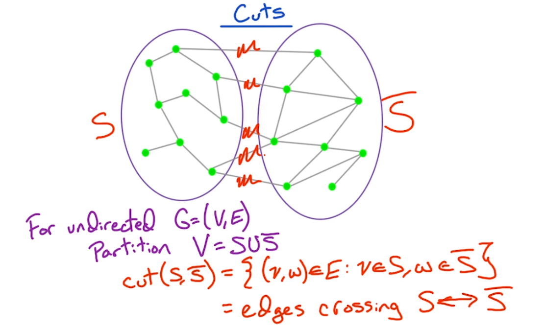
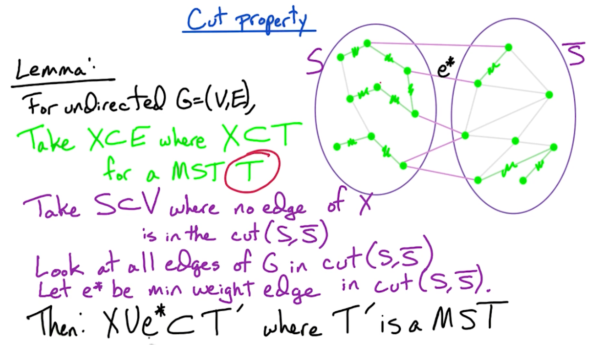
Cut property

To prove the correctness, we first need to define the cut property:

In other words, the cut of a graph is a set of edges which partition the vertices into two sets. In later part, we will look at problems such as minimum/maximum cut to partition the graphs into two components.

The core of the proof is:

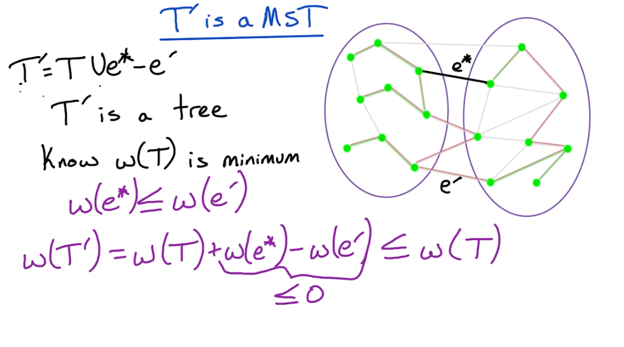
Use induction, and assume that $X \subset E$ where $X \subset T$ for a MST $T$. The claim is when we add an edge from $S, \bar{S}$, we form another MST $T’$.

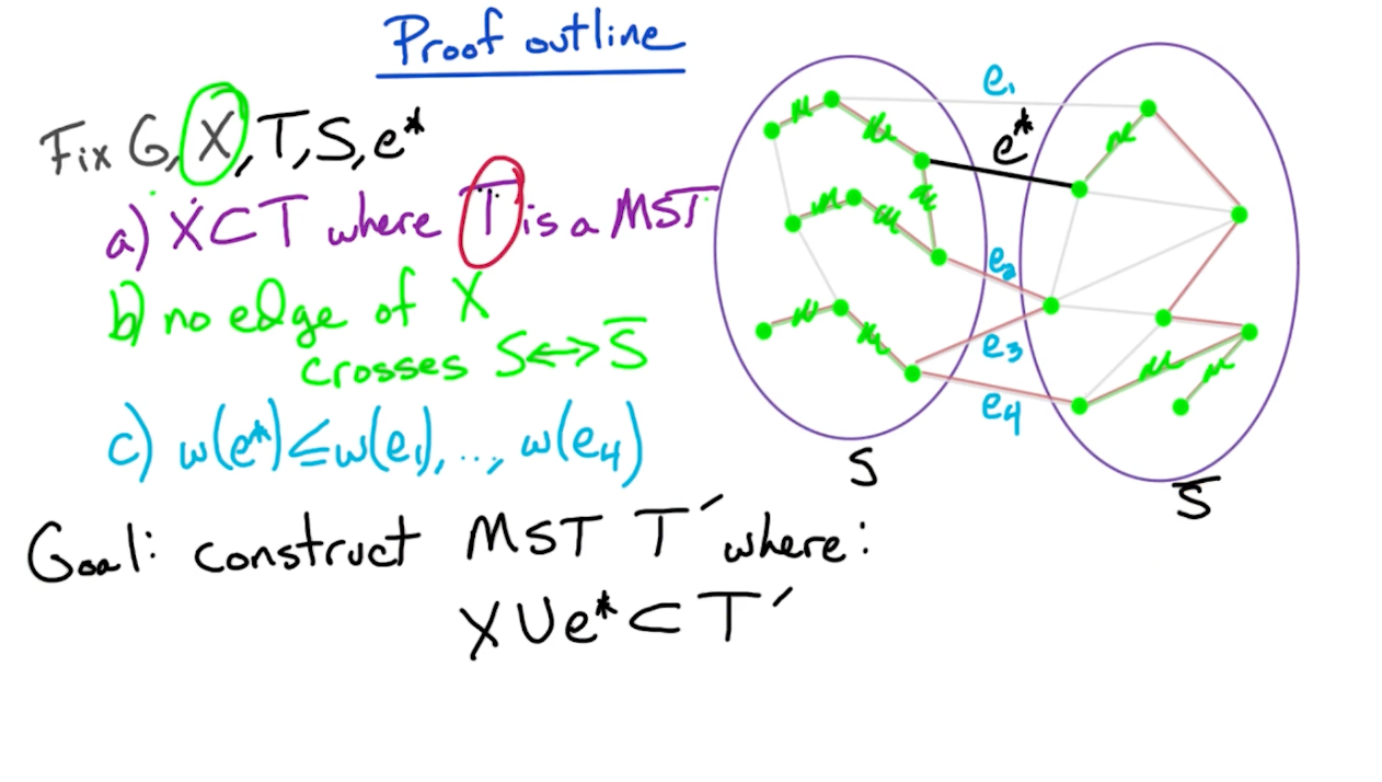
Proof outline

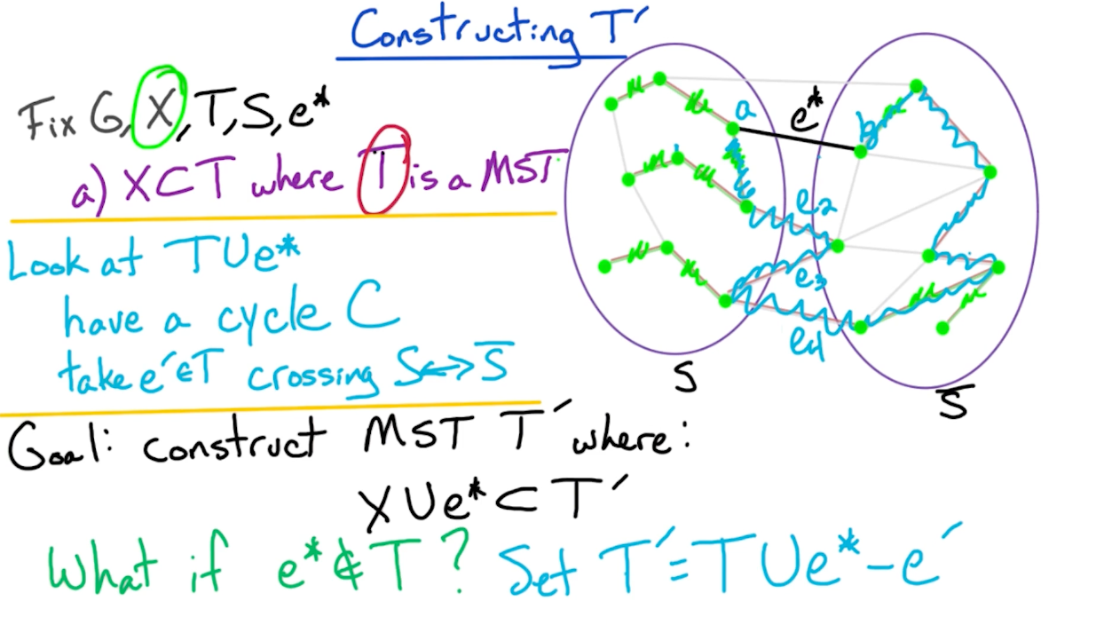
So, we need to consider two cases, if $e^* \in T$ or $e^* \notin T$.

If $e^* \in T$, our job is done, as there is nothing to show.
If $e^* \notin T$ (such as the diagram above), then we modify $T$ in order ot add edge $e^*$ and construct a new MST $T’$

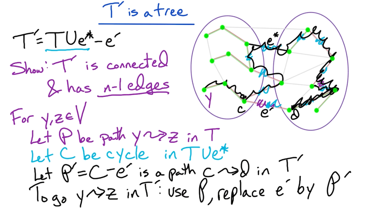
Next, we show that $T’$ is still a tree:

Remember if a tree with size $n$ has $n-1$ edges then it must be connected.

Actually, it turns out that $w(T’) = w(T)$, otherwise it would contradict the fact that $T$ is a MST.

Prim’s algorithm

MST algorithm is akin tio Dijkstra’s algorithm, and use the cut property to prove correctness of Prim’s algorithm.

The prim’s algorithm selects the root vertex in the beginning and then traverses from vertex to vertex adjacently. On the other hand, Krushal’s algorithm helps in generating the minimum spanning tree, initiating from the smallest weighted edge.

Maxflow

Ford-Fulkerson (MF1)

Problem formulation:

Input: Directed graph $G=(V,E)$ designated $s,t \in V$ for each $e \in E$, capacity $c_e >0$
Goal: Maximize flow $s \rightarrow t$, $f_e$ = flows along $e$ subjected to the following:
- Capacity constraints: * $\forall e \in E, 0\leq f_e \leq c_e$
- Conversation of flow: $\forall v \in V - {S \cup T}$, flow-in to $v$ = flow-out of $v$
- $\sum_{\overrightarrow{wv} \in E} f_{wv} = \sum_{\overleftarrow{vz} \in E} f_{vz}$

Other details:

For the max flow problems, the cycles are ok!
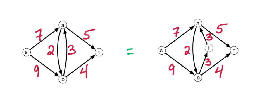
Anti parallel edges:
Notice the edge between $a\leftrightarrow b$, you want to break this anti parallel edges (Because of the residual network that we will see later)

Residual Network

Consider the following network, we initially run a path $s \rightarrow a \rightarrow b \rightarrow t$

But, it turns out that there is still capacity of $7$ left, what can we do? We build a backward edge with weights from the previous path, as shown with the red arrow below.

Now, we can pass on a flow of $7$ and the max flow is $17$.

In general, the residual network $G^f = (V,E^f)$, for flow network $G=(V,E)$ with $c_e : e \in E$, and flow $f_e : e \in E$,

if $\overrightarrow{vw} \in E\ \&\ f_{vw} < c_{vw}$, then add $\overrightarrow{vw}$ to $G^f$ with capacity $c_{vw} - f_{vw}$ (remaining available)
if $\overrightarrow{vw} \in E\ \&\ f_{vw} > 0$, then add $\overrightarrow{wv}$ to $G^f$ with capacity $f_{vw}$

In other words, if you flow is below capacity provided, add another edge in parallel with edge weight as the flow. If your flow is greater than 0 (and all capacity is used), add a backward edge with the capacity flow. Also, because we remove the parallel edges, we are allowed to add the forward edge and backward edge without inequalities.

Ford-Fulkerson Algorithm

Set $f_e = 0$ for all $ e \in E$
Build the residual network $G^f$ for the current flow $f$
- Initially it will all be zero
Check for a path $s\rightarrow t$ in $G^f$ using DFS/BFS
- If there is no such path, then output $f$.
- If there is a path, denote it a $\mathcal{P}$
Given $\mathcal{P}$, let $c(\mathcal{P})$ denote the minimum capacity along $\mathcal{P}$ in $G^f$
Augment $f$ by $c(\mathcal{P})$ units along $\mathcal{P}$
- For every forward edge, we increase the flow along that edge by this amount
- For the backward edge, we decrease the flow in the other direction
Repeat from the build residual network step (until you return output $f$)

The proof is based on max-flow = min-cut theorem, which will be covered in MF2.

For Time complexity, we assume all capacities are integers (Edmonds-Karp algorithm eliminates this assumptions). This assumption implies that whenever we augment hte flow, we augment by an integer amount.

This implies that the flow increases by $\geq 1$ unit per round
Let $C$ denote the size of max flow, then we have at most $C$ rounds.
Since the graph is connected, $\mathcal{P}$ is $n-1$ edges, so to update the residual network takes $O(n)$
To check for the path $\mathcal{P}$, either with BFS or DFS, takes $O(n+m)$, since the graph is connected, it reduces to $O(m)$.
Augment $f$ by $c(\mathcal{P})$ also takes $O(n)$
So overall the complexity of each round is $O(m)$, over $C$ rounds, hence the total runtime is $O(Cm)$.

Other Algorithms

For Ford-Fulkerson

the running time depends on the integer $C$, if you recall from knapsack, the running time is a pseudo-polynomial.
We use BFS/DFS to find any path from $s\rightarrow t$

For Edmonds-karp

Algorithm takes $O(m^2 n)$ time
We take the shortest path from $s \rightarrow t$, in this case shortest means the number of edges and do not care about the weights on the edges. To find such a path, we run BFS. The number of rounds in this case is going to be $O(mn)$, and each round takes $O(m)$ time, the total is $O(m^2n)$.
- So the runtime is independent of the max flow and no longer require it to be integer values

Orlin

$O(mn)$, generally the best for general graphs for the exact solution of the max-flow problem.

Max-Flow Min-Cut (MF2)

Recall that the Ford-Fulkerson algorithm stop when there is no more augmenting path in residual $G^{f*}$. (star here means the max flow, i.e optimal solution)

Lemma: For a flow $f^\ast$ if there is no augmenting path in $G^{f\ast}$ then $f^\ast$ is a max-flow.

Min-cut Problem

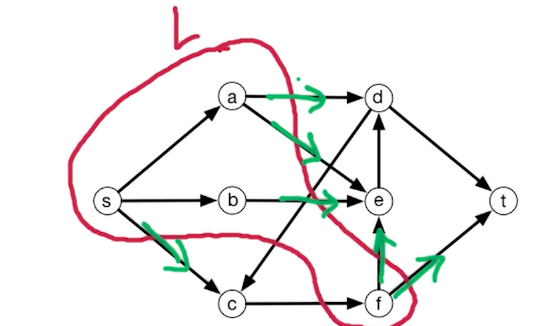
Recall that a cut is a partition of vertices $V$ into two sets, $V = L \cup R$. Define st-cut to be a cut where $s\in L, t\in R$

Notice that a cut does not need to be connected, F is not connected to A and B in this subset. We are interested in the capacity of this st-cut.

Define capacity from $L\rightarrow R$

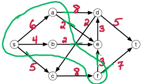
\[Capacity(L,R) = \sum_{\overrightarrow{vw} \in E: v \in L, w \in R} c_{vw}\]

Notice edges such as $C \rightarrow F$ do not count.

So the problem formulation of the min st-cut problem is as follows:

Input: flow network
Output: st-cut (L,R) with minimum capacity.

For example consider this cut, the capacity is $8+2+2+3+7+5 = 27$

The cut with minimum capacity is as follows

The min st-cut is 12, which i is equal to the max-flow 12. $L$ contains everybody but $t$. So the theorem we want to prove is the size of hte max flow equals to the size of the min st-cut.

Theorem

Note, in the max-flow problem, it is always from s to t, but on the other side it is called the st-cut problem because we want the cut to separate s and t. There could be a minimum cut such that s,t belongs to the same set.

To proof this, we show that max-flow $\leq$ min st-cut, and vice versa. This will show that max-flow == st-cut.

LHS

To show max-flow $\leq$ min st-cut, show that for any flow $f$ and any st-cut $(L,R)$:

\[size(f) \leq capacity (L,R)\]

Note - this is for any flow, which includes the max over f, and the minimum over the capacity.

Claim: $size(f) = f^{out}(L) - f^{in}(L)$

\[\begin{aligned} & f^{out}(L) - f^{in}(L) \\ &= \sum_{\overrightarrow{vw} \in E: v \in L, w \in R} f_{vw} - \sum_{\overrightarrow{wv} \in E: v \in L, w \in R} f_{wv} \\ &= \sum_{\overrightarrow{vw} \in E: v \in L, w \in R} f_{vw} - \sum_{\overrightarrow{wv} \in E: v \in L, w \in R} f_{wv} + \sum_{\overrightarrow{vw} \in E: v \in L, w \in L} f_{vw} - \sum_{\overrightarrow{wv} \in E: v \in L, w \in L} f_{wv} \end{aligned}\]

Notice that the first term and the third term, when combined, you get all edges out of v, and likewise all edges into c, and we filter out the vertex $s$. Notice that the source vertex has no input.

\[\begin{aligned} & f^{out}(L) - f^{in}(L) \\ & = \sum_{v\in L} f^{out}(v) - \sum_{v\in L} f^{in}(v) \\ & = \sum_{v\in L-S} (\underbrace{f^{out}(v)-f^{in}(v)}_{0}) + f^{out}(s) + \underbrace{f^{in}(s)}_{0}\\ &= size(f) \end{aligned}\]

So, the total flow out of $f$, is the size of $f$!. Coming back, we have:

\[size(f) = f^{out}(L) - f^{in}(L) \leq f^{out}(L) \leq capacity(L,R)\]

The last part is true, because the total flow out of L, must be the capacity out of L to R.

RHS

Now, we prove the reverse inequality:

\[max_f size(f) \geq min_{(L,R)} capacity(L,R)\]

Take flow $f^\ast$ from Ford-Fulkerson algorithm, and $f^\ast$ has no st-path in residual $G^{f\ast}$. We will construct $(L,R)$ where:

\[size(f^*) = cap(L,R)\]

Similarly, this is for any size and any capacity, we can set the left to be the max, and right to be the min:

\[max_f size(f) \geq size(f^*) = cap(L,R) \geq min_{(L,R)} capacity(L,R)\]

Take flow $f^\ast$ with no st-path in residual $G^{f\ast}$. Let $L$ be the vertices reachable from $s$ in $G^{f\ast}$. We know that $t \notin L$ because there is no such path that exists. So, let $R = V-L$. This also implies that $t \in R$.

For $\overrightarrow{vw} \in E, v\in L, w \in R$, this edge does not appear in the residual network (Because there is no path from L to R). This means that the edge must be fully capacitated $f_{vw}^* = c_{vw}$, and therefore the forward edge does not appear in the residual network so the flow along this edge equals to its capacity. Now since every edge from L to R is fully capacitated, the total flow out of $L$ must be equal to capacity$(L,R)$. This shows that $f^{*out}(L) = capacity(L,R)$.

Consider the opposite, consider edges $\overrightarrow{zy}, z \in R, y \in L$, which is edges that are going from R into L. The flow $f^\ast_{zy} = 0$ because the reverse edge does not appear in the residual network. Because if there is an edge $\overrightarrow{zy}$, then it would be reachable from $L$, then it would be included in the set $L$. Since the back edge does not appear in the residual network, then the forward edge has to have flow zero. This shows that $f^{\ast in}(L) = 0$.

Combining this two, shows:

\[size(f^*) = f^{*out}(L) - f^{*in}(L) = capacity(L,R)\]

We have shown both sides of the inequality, which concludes that max-flow == min st-cut. We have also shown that for any flow that has no augmenting path in the residual network, we can construct a st-cut where the size of the flow equals to the capacity of the s-t cut $size(f^*) = cap(L,R)$. The only way to have equality here is if both of these are optimal, which is max flow and min st-cut to have the minimum capacity.

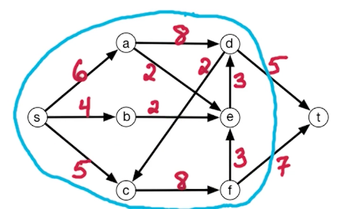
Note, this theorem also gives us another way of finding the min cut. We basically find the max flow, and set L to be all vertices reachable from s in the residual $G^{f*}$.

Edmonds-Karp (MF4)

In Ford-Fulkerson, find augmenting paths using DFS or BFS with overall run time of $O(mC)$.

In Edmonds-Karp algorithm, it finds augmenting paths using BFS, and is able to make stronger guarantees on running time, in $O(m^2n)$ and only require capacities to be positive values (no constraint on edge capacity being integer values)

The algorithm is exactly the same as Ford-Fulkerson, but we need to use BFS

Set $f_e = 0$ for all $ e \in E$
Build the residual network $G^f$ for the current flow $f$
Check for a path $s\rightarrow t$ in $G^f$ using $\cancel{DFS}$/BFS
Given $\mathcal{P}$, let $c(\mathcal{P})$ denote the minimum capacity along $\mathcal{P}$ in $G^f$
Augment $f$ by $c(\mathcal{P})$ units along $\mathcal{P}$
Repeat from the build residual network step (until you return output $f$)

Notice that the residual network has to change by at least one edge in every round. In particular, at least one edge reaches full capacity. We augment along P until we reach the full capacity of at least one edge on that path. That edge which reaches its full capacity in the residual graph, will be removed from the residual graph in the next stage. Now that edge might be a forward edge oer a backward edge, but regardless it will be removed from the residual graph in the next stage. There may be additional edges which are removed and there might be other edges which are added back into the residual network - we need some understanding of which edges are added in or removed from the residual network.

The key property remains - at least one edge is removed in every stage.

Proof

To prove that the running time is $O(m^2n)$, we show that the number of rounds is at most $mn$.

BFS takes linear time, so assuming the number of edges is at least the number of edges, so that is order $O(m)$ time per round. Combine that with $mn$ gives $O(m^2n)$

In every round, residual graph changes, at least one edge is deleted from the residual graph in every round. This edge corresponds to the one with minimum capacity along the augmenting path. Now edges may get added back in to the residual path. In particular this edge might be deleted in this round and in later rounds might be added back in.

The key lemma: for every edge $e$, we can bound the number of times that the edge is deleted in the residual graph and then reinsert it back later. In particular, $e$ is deleted and reinserted later at most $\frac{n}{2}$ times. Since there are $m$ edges in the graph and this holds for every edge of the graph, every edge is deleted at most $\frac{n}{2}$ times, and at least one edge is deleted in every round, therefore there is at most $\frac{n}{2} \times m$ total rounds. This give sour desired bound on the number of rounds of the algorithm.

Properties of BFS

BFS:

Input: directed $G=(V,E)$, no edge weights, $s \in V$
Output: for all $v \in V$, dist($v$) = min number of edges $s \rightarrow v$

The key insight here is for BFS, there is a level($v$), so the path that BFS finds from $s \rightarrow t$ is going to be a path where the level goes up by plus one at every edge, and this is the key property that we need from BFS.

So, the question is, how does level($z$) change as $G^f$ changes?

edges can get deleted! - For example in the above graph what if $\overrightarrow{AD}$ gets deleted? Does that mean the level of $d$ becomes 3?
- Need to show that when edges gets added or deleted, the level of the vertex is never going to decrease.

The claim is, for every $z \in V$, level($z$) does not decrease.

It can stay the same, or can increase in some levels, but it can never go down.

To prove this, we need to understand which edges are added into the residual network, and which edges are removed from the residual network.

How does $G^f$ change in a round? Consider each of the four cases for $\overrightarrow{vw} \in E$

Add $\overrightarrow{vw}$ if flow was full and then reduced
- So $\overrightarrow{wv} \in \mathcal{P}$
Remove $\overrightarrow{vw}$ if flow is now full
- So $\overrightarrow{vw} \in \mathcal{P}$
Add $\overrightarrow{wv}$ if flow was empty
- So $\overrightarrow{vw} \in \mathcal{P}$
Remove $\overrightarrow{wv}$ if flow was positive and now empty
- So $\overrightarrow{wv} \in \mathcal{P}$

So the conclusion is:

If add $\overrightarrow{yz}$ to $G^f$ then $\overrightarrow{zy} \in \mathcal{P}$
- This is the opposite augmenting path
If remove $\overrightarrow{yz}$ then $\overrightarrow{yz} \in \mathcal{P}$
- Edge itself is on the augmenting path

To add an edge to the residual network, we have to increase the spare capacity. That means we have to decrease the flow along this edge. To decrease the flow, then the reverse direction must be augmented.

Similarly, remove an edge from the residual graph, that means we remove the leftover capacity, in order to remove the left over capacity, that means we have to increase the flow along this edge, so the edge must be on the augmenting path $\mathcal{P}$.

Proof of Edmonds-Karp

The claim is for every $z \in V$, level($z$) does not decrease. Now, this can only happen when we add an edge which results in a shorter path. So, we ignore the case about adding edges.

Suppose level($z$) = $i$, and we add $\overrightarrow{yz}$ to $G^f$, so $\overrightarrow{zy} \in \mathcal{P}$. Any Path in Edmonds-Karp must be a BFS path, which says that the level of the vertices increase by 1 along every edge. Therefore, level($y$) = level($z$) + $1$. But notice that we are referring to the edge $\overrightarrow{yz}$, so this edge does not decrease the level of z!

What remains is the number of rounds - we need to show sometimes the level of the vertex strictly increases and this will give us a bound on the number of rounds of the algorithm.

Suppose level($v$) = $i$, and:

If we delete $\overrightarrow{vw}$ from $G^f$ so $\overrightarrow{vw} \in \mathcal{P}$
- level($w$) = level($v$) + 1 $\geq i+1$
If we later add $\overrightarrow{vw}$ into $G^f$ so $\overrightarrow{wv} \in \mathcal{P}$
- level($v$) = level($w$) + 1 $\geq i+2$

In conclusion, if we delete $\overrightarrow{vw}$ from $G^f$ and then later add $\overrightarrow{vw}$, then level($v$) increases by at least 2. The minimum level is 0, and the max level is $n$. Therefore the maximum times we can delete and add this edge back into the residual network is $\frac{n}{2}$ times, and since there are $m$ edges graphs, shows that there are at least $nm$ rounds.

Max-Flow Generalization (MF4)

Max-flow with demands

input: flow network: directed $G=(V,E)$ with $s,t \in V$ capacities $c(e) > 0, e \in E$ and demands $d(e) \geq 0, e \in E$
Output: flow is a flow $f$ where for $e \in E$, $d(e) \leq f(e) \leq c(e)$

Red represents capacity
Green represents demands
Blue is the actual flow

The goal is to find a reduction $g,f$ so we can use the max-flow algorithm. So we want to find mappings $g$ and $h$.

The intuition is we want to capture is that there is a non-negative flow along an edge, if and only if we can construct a flow in the original network.

\[\begin{aligned} f(e) \geq d(e) &\iff f'(e) \geq 0, \\ c(e) \geq f(e) &\iff c'(e) \geq f'(e) \end{aligned}\]

so this flow $f’$ is going to be a shift of $f$ by $d$ units
And also shift the capacity as well by $d$ units
- $c’(e) = c(e) - d(e)$

Consider the right graph, where the flow into a and flow out of a is zero, which is a valid flow. But if we look at the left side, that means a has an inflow of 3 units, but outflow of 8 units, which is not a valid flow since in == out. So we need to offset / fix this somehow, so a valid flow on rhs will be a valid flow on lhs.

To do this, we define $s’, t’$ where $s’ \rightarrow v, v \rightarrow t’, v \in V$.

There is still one more thing, notice that there is no flow in to $s$, so we add an edge from $s \leftarrow t$ and set it to $\infty$.

Lemma - Saturating flows

And this is the final graph $G’$ with the following:

\[\begin{aligned} D &= \sum_{e\in E} d(e) = \underbrace{\sum_{v \in V} d^{in}(v)}_{C^{ 'out}(S')} = \underbrace{\sum_{v\in V} d^{out}(v)}_{C^{'in}(t')} \\ \end{aligned}\]

For flow $f’$ in $G’$, size($f’$) $\leq D$, $f’$ is saturating if size($f’$) = $D$. This means that the flow $f’$ is of maximum size.

Lemma: $G$ has a feasible flow if and only if $G’$ has a saturating flow

If this lemma is true, then we take our feasible flow problem, construct $G’$, run max-flow on $G’$ and check if the size of the max-flow is equal to $D$ and therefore it is saturating or not. If there exists a saturating flow, implies that there is a feasible flow.

LHS (Saturating flows)

Lets show that if it is a saturating flow, then it is a feasible flow.

Take saturating flow $f’$ in $G’$, construct feasible flow $f$ in $G$, which is shifted by the demand $D$

Let $f(e) = f’(e) + d(e)$

We need to check:

$f$ is valid, flow-in = flow-out, and each edge is within capacity.
$f$ must also be feasible - satisfies all the demands constraints

To check that the demand and capacity constraints are met, and flows are non negative $f’(e) \geq 0$:

\[f'(e) \geq 0 \implies f(e) \geq d(e)\]

Then, for $G’$, each $c’(e)$:

\[c'(e) \geq f'(e) \implies f(e) \leq c'(e) + d(e) = c(e) \\ \therefore f(e) \leq c(e)\]

It remains to check that the flow is valid: $f^{in}(v) = f^{out}(v), v \in V-s-t$. Consider the graph $G’$ which is constructed with maxflow algorithm, so $f^{‘in}(v) = f^{‘out}(v)$.

\[\begin{aligned} f^{'in}(v) &= f'(\overrightarrow{s'v}) + \sum_{u\in v}\underbrace{f'(\overrightarrow{uv})}_{f'= f -d} & \text{Total flow into v} \\ &=d^{in}(v) + \sum_{u\in v} (f(\overrightarrow{uv}) - d(\overrightarrow{uv})) & \text{s'v is total demand in} \\ &=\cancel{d^{in}(v)} + \sum_{u\in v} (f(\overrightarrow{uv}) \cancel{- d(\overrightarrow{uv})}) \\ &= f^{in}(v) \end{aligned}\]

Similarly, we can show that $f^{‘out} = f^{out}$. Therefore since:

\[\begin{aligned} f^{'in}(v) &= f^{'out}(v) \\ f^{'in}(v) &= f^{in}(v) \\ f^{'out}(v) &= f^{out}(v)\\ \therefore f^{in}(v) &= f^{out}(v) \end{aligned}\]

RHS (Saturating flows)

Take a feasible flow $f$, and construct saturating $f’$ in $G’$, and we construct the feasible flow as follows:

for $e \in E$, let $f’(e) =f(e) - d(e)$
for $v \in V$:
- $f’(\overrightarrow{s’v}) = d^{in}(v)$
- $f’(\overrightarrow{vt’}) = d^{out}(v)$
- $f’(\overrightarrow{ts}) = size(f)$

We need to show that this is a valid flow. Because we assumed that $f$ is feasible, this implies (constraints are satisfied):

\[\begin{aligned} f(e) \geq d(e) &\implies f'(e) \geq 0 \\ f(e) \leq c(e) &\implies f'(e) \leq c(e) - d(e) = c'(e) \end{aligned}\]

Similarly, it remains to check $f^{‘in}(v) = f^{‘out}(v)$, this is the same as before, given that we know $f^{in}(v) = f^{out}(v)$:

\[\begin{aligned} f^{'in}(v) &= d^{in}(v) + \sum_{u\in v} (f(\overrightarrow{uv}) - d(\overrightarrow{uv})) \\ &= f^{in}(v)\\ f^{'out}(v) &= f^{out}(v)\\ \therefore f^{'in}(v) &= f^{'out}(v) \end{aligned}\]

Algorithm for feasible flow

Find a feasible flow $f$ for $G$, if one exists by checking whether the size of the max-flow equals $D$ and if it is a saturating flow. If it is, then there must be a feasible flow. Then we transform $f’ \rightarrow f$.

Then, we can augment in residual graph of $G^f$ as follows:

\[\begin{aligned} c_f({\overrightarrow{vw}})&= \begin{cases} c({\overrightarrow{vw}}) - f({\overrightarrow{vw}}) & \text{if } \overrightarrow{vw} \in E \\ f({\overrightarrow{wv}}) - d({\overrightarrow{wv}}), & \text{if } \overrightarrow{wv} \in E \\ 0, & \text{otherwise } \end{cases} \end{aligned}\]

Notice that it is a similar flow as max flow, the difference from before is that this residual graph is slightly different.

The capacity, for the forward capacity still is the capacity minus the current flow.
For reverse edges, so if there is an edge from $w$ to $v$ in the original graph, then we add the edge from $v$ to $w$ if there is flow from $w$ to $v$. Normally in residual graph, the capacity of tis reverse edge will be the flow along this edge, but now we have the constraint that the flow can never go below the demand. So the amount we can decrease the flow along this edge from $wv$ is by how much the flow exceeds the demand.

Example:

Find the flow in the following:

Solution:

The max-flow $G’$ with capacities shown:

The saturating flow:

And the solution:

Randomized algorithms

Modular Arithmetic (RA1)

Short overview of topics:

Math primer
- modular Arithmetic
- multiplicative inverses
- Euclid’s GCD algorithm
Fermat’s little theorem
- RSA algorithm
Primality testing
- is a number a prime number? or a composite number
- Generate random prime numbers

Huge integers

For huge n, consider n-bit integers, x,y, N, in the order of 1024 or even 2048 bits.

Modular Arithmetic

For integer x, x mod 2 = least significant bit of x, which tells you if x is even or odd. We can also do this by x/2 and get the remainder.

For integer $N \geq 1: x mod N$ is the remainder of x when divided by N.

Some additional notation:

\[X \equiv Y \bmod N\]

means $\frac{X}{N}, \frac{Y}{N}$ have same remainder, another way of writing this is:

\[x \bmod N = r \iff x = qN + r, q,r \in \mathbb{Z}\]

Then we have the following:

if $x \equiv y \bmod N $ and $a \equiv b \bmod N$ then $x+a \equiv y+b \bmod N$ and $xa \equiv yb \bmod N$

Modular Exponentiation

n-bit numbers, compute $x^y \bmod N$.

Consider the simple algorithm:

\[\begin{aligned} x \bmod N &= a_1 \\ x^2 \equiv a_1x \bmod N &= a_2 \\ \vdots \\ x^y = a_{y-1}x \bmod N &= a_n \end{aligned}\]

Multiplying two n-bit numbers and dividing by a n-bit number takes $O(n^2)$ per round, since we have y rounds where $y \leq 2^n$, the overall time complexity is $O(n^2 2^n)$ which is horrible

\[\begin{aligned} x \bmod N &= a_1 \\ x^2 \equiv (a_1)^2 \bmod N &= a_2 \\ x^4 \equiv (a_2)^2 \bmod N &= a_4 \\ x^8 \equiv (a_4)^2 \bmod N &= a_8 \\ \vdots \\ \end{aligned}\]

Then we can look at the binary representation of $y$ and find the appropriate $a_i$. For example if $y=25 = 11001$, then we need $a_{2^4=16} \ast a_{a^3 = 8} \ast a_{2^0=1} = a_{25}$

Mod-Exp algorithm

Note that for even $y$, $x^y = (x^{y/2})^2$, and for odd $y$, $x^y = x(x^{\lfloor y/2 \rfloor})^2$

mod-exp(x,y,N)
  Input: n-bit integers, x,y N >= 0
  Output: pow(x,y) mod N
  if y = 0, return(1)
  z = mod-exp(x, floor(y/2), N)
  if y is even:
    return (z^2 mod N)
  else:
    return (xz^2 mod N)

Multiplicative inverses

x is the multiplicative inverse of $z \bmod N$ if $xz \equiv 1 \bmod N$, which can be re-written as :

\[x \equiv z^{-1} \bmod N\]

Note that the $z$ is also the inverse of x, i.e $z \equiv x^{-1} \bmod N$

Note that the inverse is not guaranteed to exists, consider $N=14$, what is the inverse of $4 \mod 14$?

Inverse: Existence

The key idea here is if $x,N$ shares a common divisor, then it has no inverse.

Theorem: $x^{-1} \bmod N$ exists if and only if $gcd(x,N)=1$, gcd stands for greatest common divisor. This also means x and N are relatively prime.

In addition, if we always report $x^{-1} \bmod N$ in $0,1,…,N-1$ if it exists, it is unique and does not exists otherwise. For instance, $3^{-1} \equiv 4 \bmod 11$, but so is $15,26,-7$. Etc $3*-7 = -21 \bmod 11 = -1 $

Proof. Lets suppose $x^{-1} \bmod N$ has two inverses, $y \equiv x^{-1} \bmod N, z \equiv x^{-1} \bmod N, y\cancel{\equiv} z, 0 \leq y \neq z \leq N-1$.

This implies that $xy \equiv xz \equiv 1 \bmod N$. But if we multiply each by $x^{-1}$, then $x^{-1}xy \equiv x^{-1}xz \bmod N$ which implies $y \equiv z \bmod N$ which is a contradiction.

Inverse: Non existence

if $gcd(x,N) > 1$ then $x^{-1} \equiv \bmod N$ does not exists.

Lets assume $z = x^{-1} \bmod N \implies xz \equiv 1 \bmod N$ and $x,z$ shares a common divisor, $k > 1$.

This means that $xz = gN+1$, which means $akz = g(bk)+1$, for some $a$ and $b$ since $x,N$ share some common divisor $k$. But this implies that $k(az-gb) = 1$, then $az-gb = \frac{1}{k}$ which shows that $az-gb$ is a fraction but $az-gb$ is an integer since a,z,g,b are integers and $k >1$, which is a contradiction.

Euclid Rule

For integers x,y where $ x \geq y > 0$:

\[gcd(x,y) = gcd(x \bmod y ,y)\]

Proof: $gcd(x,y) = gcd(x-y,y)$, and if this is true we take x and minus y from it until we are no longer able to do so. This gives us exactly $x \bmod y$.

Now, to proof $gcd(x,y) = gcd(x-y,y)$:

if $d$ divides $x,y$ then $d$ divides $x-y$
if $d$ divides $x-y, y$, then it divides $x$ since we can just sum them up.

Euclid’s GCD algorithm

Euclid(x,y):
  input: integers (x,y) where x >= y >= 0
  output: gcd(x,y)

  if y = 0:
    return(x)
  else:
    return (Euclid(y, x mod y))

In the base case we are looking at y = 0, which is $gcd(x,0)$ What are the divisors of zero? How should we define this? What is a reasonable manner of defining the divisors of zero? Well, we got to this case by taking the GCD of sum multiple $x$ with $x$:

\[gcd(x,0) = gcd(kx, x) = x\]

Before we analyize the runtime analysis, lets prove:

Lemma: if $x \geq y$ then $x \bmod y < \frac{x}{2}$.

If $y \leq x/2$ then $x \bmod y \leq y-1 < y \leq x/2$
If $y > x/2, \lfloor \frac{x}{y}\rfloor =1$ then $x \bmod y = x-y < x - \frac{x}{2} \leq \frac{x}{2}$

Note, because of the lemma, each rounds the values decreasings by half:

\[(x,y) \rightarrow (y, x\bmod y) \rightarrow (\underbrace{x \bmod y}_{< \frac{x}{2}}, y\bmod x \bmod y ) \\ \implies 2n \text{ rounds}\]

So there is a total of $2n$ rounds. We can now do our run-time analysis.

Runtime analysis:

x mod y takes $O(N^2)$ time to compute where $N$ is the number of bits, and this is for a single round.
Total of $2n$ rounds
Total of $O(n^3)$ runtime.

Extended Euclid Algorithm

This is to compute the inverse of $x \bmod y$. Suppose $d = gcd(x,y)$ and we can express $d=x\alpha+y\beta$ and we have the following:

\[d = gcd(x,y) = d=x\alpha+y\beta\]

if $gcd(x,N) =1$ then $x^{-1} \bmod N$ exists and we have the following:

\[\begin{aligned} d = 1 &= x\alpha + N\beta \\ 1 &\equiv x\alpha + \underbrace{N\beta}_{0} \bmod N \\ x^{-1} &\equiv \alpha \bmod N \end{aligned}\]

Similarly,

\[\beta = N^{-1} \bmod X\]

Ext-Euclid(x,y)
  input: integers, x,y where x >= y >= 0
  output: integers d, α,β where d = gcd(x,y) and d = xα+yβ

  # remember gcd(x,0) = x, so we just set α = 1,β = 0
  if y = 0:
    return (x,1,0)
  else:
    d,α',β' = Ext-Euclid(y, x mod y)
    return (d, β', α' - floor(x/y)β')

The proof of the final expression can be found in the textbook, enjoy!

Runtime analysis:

Similarly, $O(n^2)$ to compute $x \bmod y$ and calculating $\lfloor \frac{x}{y} \rfloor$
$n$ rounds
Total of $O(n^3)$

Summary:

Fast Modular Exponentiation algorithm
How to calculate multiplicative inverse
- Euclid’s GCD algorithm - $gcd(x,y)$
- Extended Euclid’s algorithm to compute $x^{-1} \bmod N$

RSA (RA2)

Fermat’s little theorem

If p is prime then for every $1 \leq z \leq p-1$, so $gcd(z,p) = 1$ then:

\[z^{p-1} \equiv 1 \bmod p\]

This is the basis of RSA algorithm and also allows us to test if a number $x$ is prime.

Proof: Let $S = {1,2,3,…,p-1}, S’ = zS \bmod P = { i \times z \bmod p, i = 1, …, p-1}$.

For example $p=7,z=4, S={1,2,…,6}, S’ = {4,1,5,2,5,6}$. Notice that the sets are the same, just in different order, and we are going to use $S=S’$ to prove Fermat’s little theorem.

To proof that $S=S’$, we need to show elements of $S’$ are distinct and non zero, which implies $\lvert S’ \lvert = p-1$.

Part one - show that elements of $S’$ are distinct and we do this by contradiction, suppose for some $i \neq j$:

\[iz \equiv jz \bmod P\]

And since $P$ is a prime number, we know then that every element in $S$ has an inverse mod $P$, so $z$ is an element in S since $z$ is between a number $1, P-1$. Recall that: $P$ is prime $\implies z^{-1} \bmod p$ exists, multiplying both sides by $z^{-1}$

\[\begin{aligned} izz^{-1} &\equiv jzz^{-1} \bmod P \\ i &\equiv j \bmod P \end{aligned}\]

which is a contradiction.

Part two - Show that they are non zero. Suppose we have an index $i$ such that:

\[iz \equiv 0 \bmod P\]

and since $z^{-1}$ exists,

\[\begin{aligned} izz^{-1} &\equiv 0z^{-1} \bmod P \\ i &\equiv 0 \bmod P \end{aligned}\]

which is also a contradiction since $i$ is between $1, P-1$.

Back to the proof of Fermat’s little theorem, is to show that $z^{p-1} \equiv \bmod P$ if $P$ is prime. We have $S=S’$, then:

\[\begin{aligned} \prod_{i=1}^{P-1} i &\equiv \prod_{i=1}^{P-1} i \times z \bmod P\\ (P-1)! & \equiv z^{P-1} (P-1)! \bmod P \\ \text{Since } 1^{-1}, 2^{-1}, 3^{-1},...,&(P-1)^{-1} \text{ exists:} \\ \cancel{(P-1)!} & \equiv z^{P-1} \cancel{(P-1)!} \bmod P \\ 1 &\equiv z^{P-1} \bmod P \end{aligned}\]

Euler’s theorem

Euler theorem is the generalization of Fermat’s little theorem

For any $N,z$ where $gcd(z,N) =1$ then:

\[z^{\phi(N)} \equiv 1 \bmod N\]

where $\phi(N)$ is the number of integers between 1 and $N$ which are relatively prime to $N$, i.e the size of the set - $\lvert { x: 1\leq x \leq N, gcd(x,N) = 1} \lvert$.

$\phi$ is also known as Euler’s totient function
when $P$ is prime, then there is $P-1$ numbers relatively prime to $P$. So, $\phi(P) = P-1$.

So, for primes $p,g$ where $N=pq$, this implies that $\phi(N) = (p-1)(q-1)$

Consider $N=pq$ as $1p, 2p, … , qp$ so there are $q$ multiples of $p$.
Likewise, $q, 2q, …, pq$ there are $p$ multiples of $q$.
So, we need to exclude all these numbers!
Therefore we get $pq - p - q + 1$ which equals to $(p-1)(q-1)$
- The $+1$ comes from $pq = pq$ which is a duplicate so we need to add 1 back.

With this, we can re-write Euler theorem as the following:

\[z^{(p-1)(q-1)} \equiv 1 \bmod pq\]

And this is going to allow us to use $p-1,q-1$ to generate a encryption and decryption key.

RSA Idea

Fermat’s Theorem:

For prime $P$, take $b,c$ where $bc \equiv \bmod P-1$. This means we can re-write $bc = 1+ k(P-1)$ for some integer $k$. We then take a number $Z$ between $1$ and $P-1$:

\[\begin{aligned} z^{bc} &\equiv z^{1+K(P-1)} \bmod P \\ &\equiv z (\underbrace{z^{(P-1)}}_{1 \text{by Fermat's }})^k \bmod P \\ &\equiv z \bmod P \end{aligned}\]

The problem here is I need to tell everyone $P$, and given $b$, they are able to figure out $c$ which is the inverse of $b$ with respect to $\bmod P-1$.

Euler’s theorem:

Take $d,e$ where $de \equiv 1 \bmod (p-1)(q-1)$, and $N = pq$:

\[\begin{aligned} z^{de} &\equiv z \times (\underbrace{z^{(p-1(q-1))}}_{1})^k \bmod N \\ &\equiv z \bmod N \end{aligned}\]

Note the terms $D$ and $E$ decryption, encryption. So given a message $Z$, tell the other party $E$ and $N$:

If the other party wants to send you the message $Z$
- raise it to the power of $E$ and get $\bmod N$, i.e $z^E \bmod N$
- send it over
On my end, I compute $D$, which is the inverse of $D = E^{-1} \bmod (q-1)(p-1)$ which is my decryption key
Take the encrypted message $z^E \bmod N$, raise to the power $D$ to get $z^{DE} \bmod N$ which gives me $Z$, the original message.

Notice that the other party only knows $N$, is it possible for the other party to figure out $(p-1)$ or $(q-1)$?

Even if you tell the other party $pq$, the other party is also unable to get $(p-1)$ or $(q-1)$
But I can compute $D$ since I know $p,q$ and $E$.

Here is an image to illustrate:

Bob

Bob picks $2$ n-bit random primes $p, q$
Bob chooses $e$ relatively prime to $(p-1)(q-1)$
- Let $N=pq$ and try $e=3,5,7,11…$
- Good to keep encryption key small, easier for someone to encrypt information and send it to you.
- If you are unable to do so, usually you go back to the previous step
Bob publishes his public key $(N,e)$
Bob computes his private key
- $d \equiv e^{-1} \bmod (p-1)(q-1)$
- We can do this because of the extended Euclid algorithm.

Alice

Looks up Bob’s public key $(N,e)$
Computes $y \equiv m^e \bmod N$
- Using the fast mod-exp algorithm
Sends $y$ to bob

Bob

Bob receives $y$
Decrypts by computing $y^d \bmod N=m$
- This is because $y = m^{ed} \bmod N$
- $m^{ed} = m^{1+k(p-1)(q-1)} \bmod N$
- $m^{1+k(p-1)(q-1)} \bmod N = m \bmod N$
  - This is because of euler theorem
- This also holds when $M,N$ has a common factor namely $P$ or $Q$
  - You can still prove this statement holds with the chinese remainder theorem

Now, the question is, how do we generate this random prime number to start with?

RSA Pitfalls

Attack number one When $gcd(m,N) >1$, and $gcd(m,N) = p, N=pq$

$(m^e)^d \equiv \bmod N $ by the chinese remainder theorem
$y \equiv m^e \bmod N$
If $P$ divides $m, N$ since $gcd(m,N) = p$
- Then it is also going to divide $y$
- This means that $gcd(y,N) = p$
- The attacker can then reverse engineer $q$

Attack number two when $gcd(m,N) > 1$ and $m$ not too large, $m < N$ but $m < 2^n, N \geq 2^n$

But in this case, we $m$ cannot be too small, for example if $e=3$, then $m^3 < N$, we simply have $y = m^3$ since $\bmod N$ does nothing! To reverse the message we can simply just take the cube root.

To avoid this we can choose a random number $r$, $m\oplus r$ or $m+r$, and we can send the padded message, as well as a second message that is r itself.
- As long as r is not too small, you will be fine.
- Imagine you’re the receiving user, you receive $m+r$ and $r$, you can then reverse engineer it to get $m$

Attack number three

Send the same $m$ for $e$ times, then we have $(N_1,3), (N_2,3), (N_3,3)$.

Then we have $Y_i, \equiv m^3 \bmod N_i$ and they can figure out $m$ by using the chinese remainder theorem. (DPV 1.44)

RSA Algorithm

Choose primes $p,g$ let $N=pg$
Find $e$ where $gcd(e,(p-1)(q-1))=1$
- This means we want $e$ that is relatively prime to $(p-1)(q-1)$
- This means $e$ has an inverse by Fermat’s little theorem.
Let $d \equiv e^{-1} \bmod (p-1)(q-1)$
- Use the extended Euclid algorithm
- Keep this private key $d$ secret
Publish public key $(N,e)$
Given a message $m$, Encrypt $m$ by $y \equiv m^e \bmod N$
- Send over message $y$
Decrypt $y$ by $y^d \bmod N = m$

Why RSA is hard to break - the whole world knows $N=pq$ but only we know $(p-1)(q-1)$, and therefore only we can compute the inverse of $e^{-1} \bmod (p-1)(q-1)$

A natural question is, can you get $(p-1)(q-1)$ from $N$ without knowing $p$ and $q$ individually?
The assumption is no, it is not possible to do that. The only way to get $p-1,q-1$ is to factor $N$ into $p$ and $q$.

Random primes

let r be a random n-bit number

Choose random r 
  check if r is prime
    if yes:
      output r
    else:
      try again

A random number can be chosen by a n-bit strings.

Runtime:

Primes are dense, $Pr(\text{r is prime}) \approx \frac{1}{n}$, so you can expect to have a random prime number after $n$ tries, so, complexity here is $O(n)$.

Primality: Fermat’s test

Recall that if $r$ is prime then for all $z \in {1,. ..,r-1}$, $z^{r-1} \equiv 1\bmod r$.

So, we need to find $z$ where $z^{r-1} \cancel{\equiv} 1 \bmod r \implies r$ is composite. We call this $z$ a Fermat witness with respect to Fermat’s little theorem.

Does every composite $r$ have a Fermat witness?
- Surprisingly, YES!
How do we find one?
- In fact every composite number has multiple Fermat witness
- Some exceptions such as Pseudo Primes

Fermat Witnesses

Fermat witness for $r : z \text{ if } 1 \leq z \leq r-1 \text{ & } z^{r-1} \cancel{\equiv} 1 \bmod r$, then the number $r$ is composite.

First proof that every composite $r$ has $\geq 1$ Fermat witness. Since $r$ is composite, there is at least two divisors.

Take $z$ where $gcd(r,z) = z$ since $z \leq r-1$, and since $r$ is composite, we know this divisor is greater than one so $z > 1$. So any $z$ which is not relatively prime to $r$ and $r$ is composite will work.

This implies that $z^{-1} \bmod r$ does not exists because it only exists if and only if the $gcd(r,z) = 1$ and this is also from the inverse existence.

Suppose $z^{r-1} \equiv 1 \bmod r$, then we have $z^{r-2} \times z \equiv 1 \bmod r$, so $z^{-1} \equiv z^{r-2} \bmod r$ which is a contradiction.

Feel free to see Dpv 1.3 for more information.

Trivial Fermat witness : $z$ where $gcd(z,r) > 1$
Non-trivial Fermat witness is where $gcd(z,r) = 1$
- Some composite numbers have no non-trivial fermat witnesses, these are called pseudo primes, but those are relatively rare.
- For all other composite numbers, they have at least one non-trivial Fermat witness, and if they have at least one, they in fact have many Fermat witnesses.
- Therefore, it will be easy to find a Fermat witness
Trivial Fermat witnesses always exists!
- Every composite number has at least two trivial Fermat witnesses!
- They are dense and therefore easy to find

Non-Trivial Witnesses

$z$ is a nontrivial Fermat witness for $f$ if $z^{r-1} \cancel{\equiv} 1 \bmod r$ and $gcd(z,r)=1$.

Carmichael numbers - sort of pseudoprime numbers
- They behave like primes with respect to Fermat’s little theorem
A Carmichael number is a composite number $r$ with NO nontrivial Fermat witnesses
Such a number is going to be inefficient to use Fermat’s test to prove that $r$ is a composite number
- Find a different way to deal with them
These Carmichael numbers are rare
- smallest one are 561 and 1105, 1729 and so on
- Ignore them for now

Lemma: if $r$ has $\geq 1$ non trivial Fermat witness, then $\geq \frac{1}{2}$ that $z \in {1,2,..,r-1}$ are Fermat witness.

Proof is in the book, enjoy yourself as usual!
Question still remains, how to check a number is prime?
- Take $z$ from the set ${1,2,..,r-1}$ and raise it to the power $r-1$ and look at $\bmod r$ and see whether it is one or not.

Simple Primality tests

For n-bit r

choose z randomly from {1,2,...,r-1}
Compute pow(z, r-1) === 1 mod r
if pow(z, r-1) === 1 mod r:
  then output r is prime 
else
  output r is composite (z is a witness to the fact that r is composite)

For prime $r$, $z^{r-1} \equiv 1 \bmod r$ is true because of Fermat’s little theorem.

So Pr(algorithm outputs $r$ is prime) = 1

For composite $r$ and assume that it is not a carmichael number. Sometimes the algorithm is going to be correct, it is going to output that $r$ is composite. This happens when it finds a $z$ which is a Fermat witness. $z^{r-1} \cancel{\equiv} 1 \bmod r$

sometimes it is going to get confused, it is going to make a mistake, and it is going to find a $z$ which $z^{r-1} \equiv 1 \bmod r$, so it is going to think that $r$ is prime.
Recall that at most half of them are not witnesses
The Pr(algorithm outputs $r$ is prime) $\leq \frac{1}{2}$

The question now is, can we improve this error probability of a false positive of $\frac{1}{2}$

Better primality test

Instead of choosing a particular $z$, we choose $k-z$ and run the algorithm k times.

Then Pr(algorithm outputs $r$ is prime) $\leq (\frac{1}{2})^k$. You can think of it as a coin toss each with probability $\frac{1}{2}$. So the probability that the coin toss is all tails with k flips is $(\frac{1}{2})^k$.

So you can take $k=100$, so $(\frac{1}{2})^{100}$ is a very small number and you will be willing to take the risk on that.

Again we assume that the numbers are not Carmichael
to deal with these Carmichael, it is not that much more complicated of an algorithm

Dealing with Carmichael

So we know it is composite if there is a non trivial square root of $1 \bmod x$. Trivial square root of 1 means 1 or -1 since $1^2 , -1^2 = 1$.

For example, $x = 1729$ and choose $z = 5$, and note that $x-1 = 1728 = 2^6 \times 27$

\[\begin{aligned} 5^{27} &\equiv 1217 \bmod 1729 \\ 5^{2\times27} &\equiv 1217 \equiv 1065 \bmod 1729 \\ 5^{2^2\times27} &\equiv 1065^2 \equiv 1 \bmod 1729 \\ 5^{2^2\times27} &\equiv 1^2 \equiv 1 \bmod 1729 \\ &\vdots \\ 5^{1728} &\equiv 1 \bmod 1729 \end{aligned}\]

So, when Fermat tests fail, we see if there is a non trivial square root of 1 exists.

It turns out that for a composite number $X$, even if its Carmichael, for at least three quarters of the choices of $Z$, this algorithm works.

Nondeterministic Polynomial

Consider watching this before you start!

Definitions (NP1)

How do we prove that a problem is computationally difficult? Meaning that it is hard to devise an efficient algorithm to solve it for all inputs.

To do this, we prove that the problem is NP-complete.

Define what is NP
What exactly it means for a problem to be NP-complete

We will also look at reductions and formalize this concept of reduction.

computational complexity

What does NP-completeness mean?
What is $P=NP$ or $P\neq NP$ mean?
How do we show that a problem is intractable?
- unlikely to be solved efficiently
  - Efficient means polynomial in the input size
- To show this, we are going to prove that it is NP complete

P = NP

NP = class of all search problems. (In some courses it talks about decision problems instead which has a need for a witness for particular instances, but thats out of scope)

P = class of search problems that are solvable in polynomial time.

The rough definition is the problem where we can efficiently verify solutions, so P is a subset of NP. If I can generate solutions in polynomial time then I can also verify in polynomial time.

So if P = NP, that means I can generate a solution and verify it. If $P \neq NP$, means even if I can verify it, I might not be able to generate it.

Search Problems:

Form: Given instance I (input),
- Find a solution $S$ for $I$ if one exists
- Output NO if I has no solutions
Requirement: To be a search problem,
- If given an instance I and solution S, then we can verify S is a solution to I in polynomial time (Polynomial in $\lvert I \lvert$)

Let’s take a look at some examples

SAT problem

Input: Boolean formula in CNF with n variables and m clauses output: Satisfying assignment if one exists, NO otherwise

What is the running time to verify a SAT solution?

$O(nm)$

SAT $\in$ NP:

Given f and assignment to $x_1, …, x_n$,

$O(n)$ time to check that a clause is satisfied
$O(nm)$ total time to verify

Therefore, SAT is a search problem and therefore SAT is in NP.

Colorings

K-colorings problem:

Input: Undirected $G=(V,E)$ and integer $k > 0$ Output: Assign each vertex a color in ${1,2,…,k}$ so that adjacent vertices get different colors and NO if no such k-coloring exists

K-coloring $\in$ NP:

Given G and a coloring, in $O(m)$ time can check that for $(v,w) \in E$, color of v $\neq$ color of w.

MST

Input: $G=(V,E)$ with positive edge lengths Output: tree T with minimum weight

Is MST in the class P? - Can you generate a solution in polynomial time?

MST is a search problem
Can clearly find a solution, run Krushal’s or pim

Is MST in class NP? Can you verify a given solution in polynomial time?

Run BFS/DFS to check that T is a tree
To check if its minimum weight, run Kruskal’s or Prims to check that T has min weight.
- May output different tree, but will have the same minimum weight.
- Same runtime of $O(mlogn)$

Knapsack

Input: n objects with integer values $w_1, … , w_n$ and integer values $v_1, …, v_n$ with capacity $B$ Output: Subset S of objects with:

Total weight $\leq B$
Maximum total value

Two variants of knapsack, with and without repetition.

Is Knapsack in the class NP?

Given a solution $S$, we need to check in polynomial time that $\sum_{i \in S} w_i \leq B$. This can be done in $O(n)$ time.

The second thing to check is $\sum_{i \in S} v_i$ is optimal. Unlike MST, we cannot run the MST algorithm, and the running time for knapsack is $O(nB)$.

The runtime is not polynomial in the input size. (Not in n, logB bits)
Knapsack not known to be in NP

Knapsack is in NP, is incorrect. We do not know how to show that knapsack is in NP. Is knapsack not in NP? We cannot prove that at the moment, if we could prove that knapsack is not in NP, that would imply that P is not equal to NP. So as far as we know right now knapsack is not known to be in the class NP.

Is Knapsack in the class P? Also No.

Similarly, Knapsack is not known to be in the class P. There might be a polynomial time algorithm for knapsack, P might be equal NP in which case knapsack will lie in NP.

There is a simple variant of the knapsack problem which is in the class NP, what we are going to have to do is drop the optimization (max) and add in another input parameter.

That additional input parameter is going to be our goal for the total value and then we are going to check check whether our total value of our subset is at least the goal.
- We can do binary search on that additional parameter, the goal for the total value.

Knapsack-Search

Input: weights $w_1, …, w_n$ values $v_1, …, v_n$ with capacity B and goal g.

Output: subset S with $\sum_{i \in S} w_i \leq B$ and $\sum_{i \in S} v_i \geq g$

If no such subset $S$ exists, output NO.

Notice in the original version we are maximizing this sum of the total value, here we are simply finding a subset whose total value is at least $g$. Now, suppose that we could solve this version in polynomial time, how do we solve the maximization version?

Well, we can simply do binary search over this $g$ and by doing binary search over $g$ and we find the maximum $g$ which has a solution, then that tells us the maximum total value that we can achieve.

How many rounds in our binary search are we going to have to run? The maximum value is clearly all the items available:

\[V = \sum_{i=1}^n v_i\]

So we need to do binary search between 1 and $V$. So the total number of rounds in binary search is going to be $O(log V)$. Notice that to represent $v_1, …, v_n$ is $log v_i$ bits. So this binary search algorithm is polynomial in the input size.

Now this version can be solved in NP time, need to check in poly-time:

Given input $w_1, …, w_n, v_1, …, v_n, B, g$ and solution $S$,

$\sum_{i \in S} w_i \leq B$
$\sum_{i \in S} v_i \geq g$

Both of the above can be checked in $O(n)$ time.

Special note, you might be confused why the sum is $O(n)$ but since the input size is $log W$ and $log V$, the sum of these is still $nlogW, nlogV$ which is still in polynomial time.

P=NP revisited

P stands for polynomial time.
NP stands for nondeterministic polynomial time
- problems that can be solved in poly-time on a nondeterministic machine
- By nondeterministic time, it means it is allowed to guess at each step

The whole point of this is to tell you that NP does not meant not-polynomial time, but it is nondeterministic polynomial time.

So recall that:

NP = all search problems
P = search problems that can be solved in poly-time
- $P \subset NP$

The question now is, are there problems lie in NP which do not lie in P? That means $P\neq NP$ and there are some problems that we cannot solve in polynomial time.

NP-completeness

if $P\neq NP$ what are intractable problems? Problems that we cannot solve in polynomial time.

NP-complete problems
- Are the hardest problems in the class NP

If $P\neq NP$ then all $NP$-complete problems are not in P.

The contra positive of this statement is:

If a NP-complete problem can be solved in poly-time, then all problems in NP can be solved in poly time.

Hence to show a problem such as SAT, we have to show that if there is a polynomial time algorithm for SAT then there is a polynomial time algorithm for all problems in the class NP.

To do that, we are going to take every problem in the class NP, and for each of these problems have a reduction to SAT.
- If we can solve SAT in polynomial time, we can solve every such problem in class NP in polynomial time.

SAT is NP-complete

SAT is NP-complete means:

SAT $\in$ NP
If we can solve SAT in poly-time, then we can solve every problem in NP in poly-time.

Reduce all problems to SAT!

If $P\neq NP$ then SAT $\notin$ $P$, then we know that there are some problems in NP which cannot be solved in polynomial time, and therefore we cannot solve SAT in poly-time.

Because if we can solve SAT in poly-time then we can solve all problems in NP in polynomial time.
Or if you believe that nobody knows how to prove that $P=NP$ then nobody knows a polynomial time algorithm for SAT.

It might occur to you that a polynomial time to solve SAT does not exists, otherwise we would have proven $P=NP$!

Reduction

For problems A and B, a reduction of can be represented as:

$A \rightarrow B$
$A \leq B$

Means we are showing that B is at least as hard computationally as A, i.e if we can solve B, then we can solve A.

If we can solve problem B in poly-time, then we can use that algorithm to solve A in poly-time.

How to do a reduction

Colorings $\rightarrow$ SAT

Suppose there is a poly-time algorithm for SAT and use it to get a poly-time algo for Colorings.

You can take any problem $I$, map it with $f$, and use SAT algorithm, get the results and map it back with $h$. If solution does not exists, just return NO.

So we need to define $f, h$

$f$ : input for colorings $(G,k) \rightarrow$ input for SAT, $f(G,k)$
$h$ : solution for $f(G,k)$ $\rightarrow$ solution for colorings

Need to prove that if $S$ is a solution to $f$, then $h(S)$ is a solution to the original $G$. But we also need that if there was no solution to $f$, then there is no solution to the colorings problem.

$S$ is a solution to $f(G,k) \iff h(S)$ is a solution to $(G,k)$.

NP-completeless proof

To show: Independent sets is NP-complete

Independent Sets (IS) $\in$ NP
- Solution can be verified in polynomial time
$\forall A \in NP, A\rightarrow IS$
- Reduction of A to Independent Sets

Suppose we know SAT is NP-complete, $\forall A\in NP, A\rightarrow \text{ SAT}$, if we show

\[\begin{aligned} \text{SAT} \rightarrow \text{IS} &\implies A \rightarrow {SAT} \rightarrow \text{IS}\\ &\implies A \rightarrow \text{IS} \end{aligned}\]

Instead, to show IS is NP-complete, we need:

IS $\in$ NP
SAT $\rightarrow$ IS

3SAT (NP2)

The SAT is NP-complete, and known as the Cook-Levin Theorem (71). It was proved independently in 1971 by Steven Cook and Leonid Levin.

Karp’72 - 21 other problems are NP-complete

3SAT

Input: Boolean formula $f$ in CNF with n variables and m clauses where each clause has $\leq$ e literals

Output: Satisfying assignment, if one exists & No otherwise.

Now, to show that 3SAT is NP-complete, need to show:

3SAT $\in$ NP
SAT $\rightarrow$ 3SAT

Why do we care about this? Because if we an do this, then:

\[\forall A\in \text{ NP}, A \rightarrow \text{ 3SAT}\]

The implications is that if we have a polynomial time algorithm for 3SAT, then we have a polynomial time algorithm for every problem in NP, because we can reduce every problem in NP to 3SAT.

3SAT in NP

Given 3SAT input $f$ and T/F assignments for $x_1, …, x_n$. We want to show that 3SAT $\in$ NP.

To verify this assignment is a Satisfying assignment:

For each clause $C\in f$ in $O(1)$ time can check that at least one literal in $C$ is satisfied.
- Order $O(1)$ time per clause, there are $M$ clauses so takes total $O(m)$ time.
- It is $O(1)$ because fixed number of literals per clause.

SAT reduces to 3SAT

To do so, we need to take input $f$ for SAT:

Need to create $f’$ for 3SAT
Transform satisfying $\sigma’$ for $f’ \rightarrow \sigma$ for $f$
- $\sigma’$ satisfies $f’ \iff \sigma$ satisfies $f$

Example:

\[f = (x_3) \land (\bar{x_2} \lor x_3 \lor \bar{x_1} \lor \bar{x_4}) \land (x_2 \lor x_1)\]

We can re-write $C_2 = (\bar{x_2} \lor x_3 \lor \bar{x_1} \lor \bar{x_4})$ as:

\[C'_2 = (\bar{x_2} \lor x_3 \lor y ) \land (\bar{y} \lor \bar{x_1} \lor \bar{x_4})\]

The claim is $C_2$ is satisfiable $\iff$ $C’_2$ is satisfiable

Forward direction, take satisfying assignment for $C_2$:

if $x_2=F$ or $x_3 = T$ then set $y=F$
if $x_1=F$ or $x_4 = F$ then set $y=T$

Backwards direction, take satisfying assignment for $C’_2$

if $y=T$ then $x_1 = F$ or $x_4 = F$
if $y=F$, then $x_2=F$ or $x_3=T$

Big Clauses

Given $C=(a_1 \lor a_2 \lor … \lor a_k)$ where $a_1, …, a_k$ are literals:

Create $k-3$ new variables, $Y_1, Y_2, …, Y_{k-3}$
Note that these variables are distinct for each clause, so if you have 2 clauses you will have two sets of new variables
- So if you have $n$ clauses with $m$ literals then you have have order $nm$ new variables

\[C' = (a_1 \lor a_2 \lor y_1) \land (\bar{y_1} \lor a_3 \lor y_2) \land (\bar{y_2} \lor a_4 \lor y_3) \land \\ ... \land (\bar{y_{k-4}} \lor a_{k-2} \lor y_{k-3}) \land (\bar{y_{k-3}} \lor a_{k-1} \lor a_k)\]

Now we need to show that $C$ is satisfiable $\iff$ $C’$ is satisfiable.

Forward implication: Take assignment to $a_1,…,a_k$ satisfying $C$.

Let $a_i$ be minimum $i$ where $a_i$ is satisfied.

Since $a_i = T \implies (i-1)^{st}$ clause of $C’$ is satisfied.
- e.g if $a_i = a_4$ then $(\bar{y_2} \lor a_4 \lor y_3)$ is satisfied
  - It has $i=4$ which is the $i-1=3$ term
Set $y_1=y_2=…=y_{i-2} = T$ to satisfy $1^{st} (i-2)$
Set $y_{i-1} = y_i = … = y_{k-2} = F$ to satisfy rest

Reverse implication, take assignment to $a_1, …, a_k, y_1, …, y_{k-3}$ satisfying $C’$

Suppose at least one $a_i = T$, then we can just use the original $a_i$
Suppose otherwise $a_1 = a_2 = … = a_k = F$, we will show it is not possible to satisfy $C$.
- From clause $1 \implies y_1 = T$
- From clause $2 \implies y_2 = T$
- $…$
- From clause $k-3 \implies y_{k-3} = T$
$(\bar{y_{k-3}} \lor a_{k-1} \lor a_k)$ but this last literal is not set to true, it is all False. So the entire C is evaluated to be False.

SAT reduces to 3SAT cont

SAT->3SAT
Consider f for SAT
Consider f' for 3SAT:
  For each clause C in f:
    if |C| <= 3 then:
      add C to f'
    if |C| > 3 then:
      create k-3 new variables 
      and add C' as defined as before

It remains to show that $f$ is satisfiable $\iff$ $f’$ is satisfiable.

Then, we need to show given a satisfying assignment to $f’$, how to map it back to $f$.
- That will be straight forward because we just ignore these auxiliary variables and the setting for the original variables will give us a satisfying assignment to the original form.

Correctness of SAT->3SAT

$f$ is satisfiable $\iff$ $f’$ is satisfiable

Forward direction: Given assignment $x_1,…,x_n$ satisfying $f$

If $\lvert C \lvert \leq 3$ then we simply ignore it, otherwise:
Remember that for each C, we define a new set $K-3$ of variables.
- There is an assignment $k-3$ new variables so that $C’$ is satisfied

Backward direction: Given satisfying assignment for $f’$

For $C’ \in f \geq 1$ literal in C is satisfied
- Otherwise there would be no way to satisfy this sequence of clauses $C’$
Ignore the new variables and just look at the setting on the original n variables

Satisfying assignment

Now, how do we get the mapping back?

That is, we need transform our SAT assignment $\sigma’$ for $f’$ and get back $\sigma$, the SAT assignment for $f$

We can ignore the assignment for the new variables and keep the assignment for the original variables the same, then we get a satisfying assignment for $f$. So we take this satisfying assignment for $f$ prime, we ignore this assignment for all of the new variables and the assignment for the original variables gives us a satisfying assignment for $f$. And that completes our reduction.

Size of problem?

$f$ has n variables, $m$ clauses.

$f’$ has $O(nm)$ variables in the worst case
We are also replacing every clause by order $n$ clauses.
So we also have $O(nm)$ clauses

But this is ok! Because the size of $f’$ is polynomial in the size of $f$. So we have an algorithm which is polynomial running time in the size of $f’$.

Graph Problems (NP3)

Independent sets
Clique
Vertex cover

Independent Set

For undirected $G=(V,E)$, subset $S \subset V$ is an independent set if no edges are contained in $S$. i.e for all $x,y \in S, (x,y) \notin E$

An example:

Another example:

Trivial to find small independent sets:

Empty set
Singleton vertex

Challenging problem is to find the max independent set.

Question: The maximum independent set problem is known to be in NP, True or False?

If you give me a solution, no way to verify that it is, in fact, of maximum size.
The only way to verify if it is of maximum size is it if I can solve this problem in polynomial time.
- Only holds if $P=NP$
Assuming $P\neq NP$, the max independent set is not in the class NP.
- Similar scenario for the optimization version of knapsack problem

Max independent set

Input: undirected $G=(V,E)$ and goal g

Output: independent set $S$ with size $\lvert S \lvert \geq g$ and NO otherwise.

Theorem: The independent set problem is NP-complete.

Need to show:

Independent Set $\in$ NP
- Given input $G,g$ and solution $S$, verify that $S$ is a solution in polynomial time.
- in $O(n^2)$ time can check all pairs $x,y \in S$ and verify $(x,y) \notin E$
- in $O(n)$ time can check $\lvert S \lvert \geq g$
Need to show that the independent set is at least as hard as every problem in the class NP.
- Take something which is known to be at least as hard as everything in the class NP such as SAT or 3SAT.
- Show a reduction from that known NP-complete problem to this new problem.
- Show that $3SAT \rightarrow \text{Independent Set}$

3SAT is considered instead of SAT because it is easier.

3SAT -> IS

Consider 3SAT input $f$ with variables $x_1,…,x_n$ and clauses $C_1,…,c_m$ with each $\lvert C_i \lvert \leq 3$. Define a graph G and set $g=m$.

Idea: For each clause $C_i$, create $\lvert C_i \lvert$ vertices.

Since there are $m$ clauses, there is at most $3m$ vertices in graph $G$
Going to add edges to encode this clause.
Add additional edges between vertices in different clauses in order to ensure consistent assignment

Clauses edges

Two types of edges, Clauses and Variables.

Clause $C = (x_1 \lor \bar{x_3} \lor x_2)$

If another vertices shares $x_2$, we will have another vertex corresponding to $x_2$, multiple vertices corresponding to the same literal.

Independent set $S$ has $\leq 1$ vertex per clause. Since $g=m$, solution has $=1$ vertex per clause.

Since every independent set has at most one vertex per clause, in order to achieve our goal of an independent set of at least $m$, this solution has to have exactly one vertex per clause.

This one vertex per clause will correspond to this satisfied literal in that clause. Now there may be other satisfied literals in the clause due to other copies of that literal in other clauses, but this property that we have exactly one vertex per clause will ensure that we have at least one satisfied literal in every clause, and therefore, this solution, this independent set will be able to relate it to a satisfying assignment for this original formula.

Now, what happens if i take an independent set containing $x_1$ and $\bar{x_1}$, well in the above graph, this is in fact an independent set in this graph. And it can take one of $x_4, x_5$ and then I can have my independent set of my goal size of three. Now a natural way of converting this independent set into an assignment for the original formula is to satisfy each of the corresponding literals.

So we set $x_1 =T$, $x_5=T$, $\bar{x_1} = F$ but this arrives at a contradiction. How do we ensure that my independent sets correspond to valid assignments?

Variable edges

For each $x_i$, add edges between $x_i$ and all $\bar{x_i}$

This will ensure that our independent set corresponds to a valid assignment. And then the clause edges will ensure that our independent set corresponds to an assignment which satisfies all the clauses.

Example

Now an example independent set of size four in this graph:

Note that $z$ has no constraints.

Now lets prove that in general, that an independent set of size $m$ in this graph corresponds to a satisfying assignment of this formula, and a satisfying assignment of this formula corresponds to an independent set of size $m$.

Correctness 3SAT -> IS

$f$ has a satisfying assignment $\iff$ $G$ has an independent set of size $\geq g$

Forward direction: Consider a satisfying assignment for $f$ and we will construct an independent set in this graph of size at least $g$.

For each clause $C$ at least one of the literals and that clause is satisfied, take 1 of the satisfied literals, add corresponding vertex to $S$.

$S$ contains exactly one vertex per clause.
So $\lvert S \lvert =m = g$, and our goal $g$ is met.

Since $S$ contains exactly one vertex per clause, and it never contains both $x_i, \bar{x_i}$. It cannot contain both since it corresponds to an assignment $f$, which sets either $x_i$ to be true or false. Because there is at most one vertex per clause, we know that there is no clause edges contained in this set $S$ and because we never include a vertex $x_i, \bar{x_i}$ in the assignment, we know that there are no variable edges contained in this set $S$.

Therefore, S is an independent set of size equal to $g$, our goal size. So we have constructed an independent set of size equal to $g$ in this graph.

Backward direction: Take independent set $S$ of size $\geq g$ has exactly one vertex in each of the clauses, actually in each of the triangles corresponding to the clauses.

Now this vertex corresponds to a literal in the original formula so we set that corresponding literal to true.
Since every clause has a satisfied literal then we know every clause is satisfied and therefore the formula is satisfied. But does this clause belongs to an assignment?

Notice we have no contradicting literal in this set since we added edges between $x_i, \bar{x_i}$ so we can never include $x_i$ and a $\bar{x_i}$ in an independent set. Therefore we never attempt to set $x_i$ to be true and false at the same time. So this assignment we constructed corresponds to a valid assignment.

So we taken an independent set of size at least $g$ and we construct a satisfying assignment.

This proves that a reduction from 3SAT to independent set is correct and it shows how to take an independent set and construct a satisfying assignment. And if there is no independent set of size at least $g$ then there is no satisfying assignment.

This completes the proof that the independent set problem is NP-complete.

NP-HARD

In the Max-independent set problem, it is not known to lie in the class NP. Notice that it is quite straight forward to reduce the independent set problem to max independent set problem. I am looking for an independent set of size at least $g$, while on the other side is looking for maximum independent set. IF i find the max independent set, and i check whether that size is at least $g$, that either gives me a solution or tells me there is no solution.

So it is quite forward to reduce the search version to the optimization version. That means I have reduction from the independent set problem to the maximum independent set problem and in fact, I have a reduction from every problem in NP to the MAX independent set problem. Either going indirectly through or directly.

Theorem: The Max-Independent Set problem is NP-hard

NP-hard means it is at least as hard as everything in the class NP. So there is a reduction from everything in the class NP to this problem max independent set. So if we can solve max independent set in polynomial time, then we can solve everything in NP in polynomial to be NP-complete.

Clique

For undirected graphs, $G=(V,E)$, $S\subset V$ is a clique if:

for all $x,y \in S, (x,y) \in E$
- All pairs of vertices in the subset $S$ are connected by an edge.

Want large cliques, small cliques are easy to find:

For an example the empty set
Singleton vertex
Any edge (with two end points)

Now, let’s defined the clique problem:

Input: $G=(V,E)$ and goal $g$

Output: $S \subset V$ where $S$ is a clique of size $\lvert S \lvert \geq g$ if one exists, No otherwise.

Find the largest clique possible

Theorem: The clique problem is NP complete

Clique $\in$ NP

Given input $(G,g)$ and solution $S$.
For all $x,y \in S$, check that $(x,y) \in E$
- At most takes $O(n^2)$ for each pair
- At most $O(n)$ time to check whether they are connected by an edge
- Total of $O(n^3)$ with a trivial algorithm
  - You could do it easily in $O(n^2)$ as well
Check that $\lvert S \lvert \geq g$
- Order $O(n)$ time

Now, we need to show that the clique problem is at least as hard as other NP problems. We show reduction from a known NP-complete problem to the clique problem

Choices are SAT, 3SAT, IS - take the one most similar to clique, Independent Sets which is also a graph problem

IS -> Clique

The key idea is for clique, it is all edges within $S$, while independent set is no edges within $S$. So, they are actually opposite of each other.

For $G=(V,E)$ transform the input for the independent set for the clique problem. We can take the opposite of $G$, denoted as $\bar{G}$

Let $\bar{G} = (V, \bar{E})$ where: $\bar{E} = { (X,y) : (x,y) \notin E}$

Observation: $S$ is a clique in $\bar{G} \iff$ $S$ is an independent set in $G$

Recall that for independent sets, all pairs of vertices are not connected by an edge, which is the opposite for a clique.

IS $\rightarrow$ clique:

Given input $G=(V,E)$ and goal $g$ for IS problem, let $\bar{G},g$ be input to the clique problem.

If we get solution $S$ for clique, then return $S$ for IS problem
If we get NO, then return NO.

Vertex cover

$S \subset V$ is a vertex cover if it “covers ever edge”

For every $(x,y) \in E$ either $x \in S$ and/or $y\in S$.

It is easy to find a large vertex cover, i.e all vertices in the vertex cover, but in this case we are trying to find the minimum vertex cover.

Input: $G=(V,E)$ and budget $b$

Output: vertex cover $S$ of size $\lvert S \lvert \leq b$ if one exists, NO otherwise.

Theorem: vertex cover problem is NP-complete

Vertex Cover $\in$ NP

Given input $(G,b)$ and proposed solution $S$, can we verify this in polynomial time?
- For every $(x,y) \in E, \geq 1$ of $x$ or $y$ are in $S$
  - Can be done in $O(n+m)$ time
- Check that $\lvert S \lvert \leq b$
  - Can be done in $O(n)$ time

Now, we need to take independent set problem and reduce it to vertex cover

The claim is $S$ is a vertex cover $\iff$ $\bar{S}$ is an independent set

Forward direction:

Take vertex cover $S$, for edge $(x,y) \in E: \geq 1$ of $x$ or $y$ are in $S$.

Therefore $\leq 1$ of $x$ or $y$ in $\bar{S}$
- $\implies$ no edge contained in $\bar{S}$ since it only contains $x$ or $y$, so does not have the edge $(x,y)$
Thus $\bar{S}$ is an independent set

Reverse direction:

Take independent set $\bar{S}$

For every $(x,y)$, $\leq 1$ of $x$ or $y$ in $\bar{S}$
- implies that $\geq 1$ of $x$ or $y$ in $S$
- $\therefore S$ covers every edge

IS -> Vertex cover

Claim: $S$ is a vertex cover $\iff$ $\bar{S}$ is an independent set

For input $G=(V,E)$ and $g$ for independent set

Let $b=n-g$
- Run vertex cover on $G,b$

$G$ has a vertex cover of size $\leq n-g \iff G$ has an independent set of size $\geq g$

So now we have:

$(G,g)$ for independent set $\rightarrow$ $(G,b)$ for vertex cover.

Given solution $S$ for vertex cover, return $\bar{S}$ as solution to independent set problem
- We know that if $S$ is a vertex cover of size at most $b$, then we know that $\bar{S}$ is an independent set of size at least $g$
If NO solution for VC return NO for IS problem.

Knapsack (NP4)

Subset-sum

Input: positive integers $a_1, …, a_n, t$

Output: Subset $S$ of ${1, …, n}$ where $\sum_{i \in S} a_i = t$ if such a subset exists, NO otherwise.

If using dynamic programming, we can solve this in $O(nt)$

This is not in P because this is the same as knapsack, the running time has to be $O(nlogt)$

Subset-sum is NP-complete

First show that subset-sum $\in$ NP.

Given inputs $a_1,…,a_n, t$ and $S$, check that $\sum_{i \in S} a_i = t$.

To compute this sum, there are are most $n$ numbers, and each number is at most $log t$ bits, so the total takes $O(nlogt)$. This is polynomial in input size.

Now we need to show the second part, is at least as hard as every problem in class NP. We are going to use the 3SAT problem.

The reduction will really illustrates why the order $O(nt)$ time algorithm is not efficient for this subset-sum problem.

3SAT -> Subset sum

Input to subset-sum: $2n+2m+1$ numbers:

$v_1, v_1’, v_2, v_2’, …, v_n, v_n’, s_1, s_1’, …,s_m, s_m’$ and $t$
- $v_i’$ represents $\bar{x_i}$ and $s$ represents each clause.
- $n$ for the number of literals
- $t$ represents the desired sum

All these numbers are huge, all are $\leq n+m$ digits long and we are going to work in base 10.

This is so that if we add up any subset of numbers, there will be no carries between the digits.
This means $t \approx 10^{n+m}$

Lets take a deeper look:

$v_i$ corresponds to $x_i$: $v_i \in S \iff x_i = T$
$v_i’$ corresponds to $x_i$: $v_i \in S \iff x_i = F$

And assignment for the 3-SAT formula either sets $x_i$ to True or False. Therefore we need for the subset sum problem that either we include $v_i \in S$ or $v_i’ \in S$, but we cannot include both and cannot include neither otherwise there is no assignment for $x_i$.

To achieve this, in $i^{th}$ digit of $v_i, v_i’, t$, put a $1$ and all other numbers put a 0. Now by using base 10, we will ensure that there is no carries between the digits. So each digit is going to behave independently. REcall that $t$ is our desired sum, so the only way to achieve a desired sum that has a one in the $i^{th}$ digit is to either include $v_i$ or $v_i’ \in S$, not both and not neither.

This specification ensures that our solution to the subset sum problem is going to correspond to an assignment. Whether it is satisfying or not is another issue.

Example Reduction:

From here, Digit $n+j$ corresponds to clause $C_j$.

if $x_i \in C_j$ put a 1 in digit $n+j$ for $v_i$.
if $\bar{x_i} \in C_j$ put a 1 in digit $n+j$ for $v_i’$.
Put a 3 in digit $n+j$ of $t$
Use $s_j,s_j’$ to be buffer
- put a 1 in digit $n+j$ of $s_j, s_j’$
Put a 0 in digit $n+j$ of other numbers

Take $C_1$ for example, we set $S_1, S_1’$ to also be $1$.

So to get 3, we need at least one $v_i$ to be $1$.

Correctness Subset sum

Now is to prove that subset-sum has a solution $\iff$ 3SAT $f$ is satisfiable

Forward direction:

Take solution $S$ to subset sum:

For digit $i$ where $1\leq i \leq n$, to get a 1 in digit $i$, to include $v_i$ or $v_i’$ but not both (or neither)
So the only way to get a sum of exactly 1 in digit $i$ is to include exactly
- If $v_i \in S$ then $x_i = T$
- If $v_i’ \in S$ then $x_i = F$
$\implies$ get an assignment

Now we need to show that this assignment is a satisfying assignment

For digit $n+j$ where $1\leq j \leq m$
- Corresponds to clause $C_j$
- To get a sum of 3 in digit $n+j$:
  - Need to use $\geq 1$ literal of $C_j$ and include $S_j, S_j’$
    - If we have two $C_j$ we just need to use either $S_j$, $S_j’$ and so on.
    - If we satisfy all three $C_j$ then don’t need either
    - If none are satisfied there is no way to achieve a sum of 3, therefore no solution exists
- $\implies C_j$ is satisfied

Backward direction:

Take a satisfying assignment for $f$ and construct a solution to the subset-sum instance in the following manner:

If $x_i = T$, add $v_i$ to $S$
If $x_i = F$, add $v_i’$ to $S$
- $\implies i^{th}$ digit of $t$ is correct
For clause $C_j$, at least 1 literal in $C_j$ is satisfied
- The numbers corresponding to these literals gives us a sum one, two or three in the digit $n+j$.
  - To get a sum of $3$ in digit $n+j$, use the numbers corresponding to these literals use $S_j,S_j’$ to get up to the sum of three.
- This ensures that digit $n+j$ is correct and therefore the last $m$ digits are correct and the first $n$ digits are correct.
Therefore we have a solution to the subset-sum instance

Knapsack is NP-complete

Prove that the knapsack problem is NP-complete.

Use the correct version of the knapsack problem, the version which lies in the class NP.

As before, there is two parts:

Knapsack $\in$ NP
Known NP-complete problem $\rightarrow$ knapsack

We know that all problems in NP reduce to this known NP-complete problem, therefore if we show a reduction from this known NP-complete problem to the knapsack problem, we know all NP problems can reduce to the knapsack problem.

Try to use the subset-sum to show this

Halting Problem (NP5)

Undecidability

NP-complete means it is computationally difficult, if P $\neq$ NP, no algorithm which takes poly-time on every inputs.

Undecidable means it is computationally impossible, no algorithm solves the problem on every input regardless of the running time (or space) of the algorithm.

In 1936, Alan Turing prove that the halting problem is undecidable!

Halting problem

Input: A program $P$ (in any language) with an input $I$

Output: True if $P(I)$ ever terminates, False if $P(I)$ never terminates (i.e has an infinite loop)

For example, consider a program P:

while x mod 2 == 1:
    x +=  6

If x is initially set to 5, then this program never halts.

HP: undecidable

Theorem: The halting problem is undecidable.

We prove this by contradiction, suppose we had an algorithm that solves the halting problem on every input, call this algorithm the Terminator(P,I). We construct a new program Q and input J, show that Terminator(Q,J) is incorrect.

Since Terminator is incorrect on this pair of inputs, therefore, Terminator does not solve the halting problem on every input which is a contradiction.

Notice that we are assuming the existence of this Terminator program! We can use it as a subroutine, a black box.

HP: paradox

Consider the following “evil” program:

Harmful(J):
   (1)if Terminator(J,J):
        then GOTO(1)
      else Return() 

Dijkstra - Goto statement considered harmful (Feel free to google this)

The harmful program is just an if then else statement, takes an input J, and run Terminator(J,J). So J is a program and J is the input to the program J.

If Terminator returns true on this input pair then our program goes to one, so we get this loop. If Terminator returns false, then we simply exit the procedure and we exit the program harmful.

HP: What’s harmful?

Terminator(J,J): Runs program on input J

Returns True if J(J) terminates
Returns False if J(J) never terminates

Therefore:

If J(J) terminates then Harmful(J) never terminates
If J(J) never terminates then Harmful(J) terminates

HP: paradox

To arrive at our paradox, we set input J = Harmful which we just defined.

The question is does Harmful(Harmful) terminate when it takes itself as an input?

So lets consider the two cases and plugging in our above statements when J = Harmful,

If Harmful(Harmful) terminates, then Harmful(Harmful) never terminates
- This is a contradiction and this cannot be the case.
If Harmful(Harmful) never terminates, then Harmful(Harmful) terminates
- But this is also a contradiction

Therefore, the assumption that Terminator() exists is impossible! Our initial assumption that the program Terminator which solves the halting problem on every input exists must be impossible

Linear programming

Linear Programming (LA1)

Will look at simple examples such as:

max-flow
simple production

Will look at standard form, and LP duality.

Maxflow via LP

Input: Directed $G=(V,E)$ with capacities $c_e > 0$ for $e \in E$

LP: $m$ variables: $f_e$ for every $e \in E$

Objective function: $max \sum_{\overrightarrow{SV} \in E} f_{sv}$

Subject to:

for every $e \in E, 0 \leq f_e \leq c_e$
For every $v\in V-{s,t}$, $\sum_{\overrightarrow{wv}\in E} f_{wv} = \sum_{\overrightarrow{vz}\in E} f_{vz}$

This should look familiar, which is the feasibility of a flow.

2D example

Company makes A and B, how many of each to maximize profit?

Each unit of A makes profit of $1, B makes $6
Demand: $\leq 300$ units of A and $\leq 200$ units of B
Supply: $\leq 700$ hours, A takes 1 hour, and B takes 3 hours.

To express this as a linear program:

Variables: let $x_1, x_2$ be the number of units of A and B respectively
Objective function: max $x_1 + 6x_2$
Demand: $0\leq x_1 \leq 300, 0\leq x_2 \leq 200$
Supply: $x_1+3x_2 \leq 700$

Feasible Region - all possible solutions:

Finding the best solution involves drawing a line $x_1+6x_2$ and slowly moving up, something like sliding up a roller.

In the above scenario, it touches the point $(100,200)$, so $x_1 = 100, x_2 = 200$

There a few key points:

Optimum may be non-integer
- We can round it - Will revisit this in Max-Set Approximation algorithm
$LP \in P$
- But Integer Linear Programming (ILP) is NP-complete
Optimal solution lies in a vertex (corner)
Feasible region is convex
- All points between two lines must be in the set
  - Optimal point at vertex
  - The whole line may be optimal, but it must end somewhere at a vertex / corner
- If a vertex is better than its neighbors, it is the global optima

This gives rise to the simplex algorithm which we will detail later.

3D example

Profit: 1 for A, 6 for B, 10 for C.
Demand: $\leq 300$ for A, $\leq 200$ for B, unlimited demand for C
supply $\leq 1000$ A takes 1, B takes 3, C takes 2
Packaging $\leq 500$ total, A requires no packaging, B takes 1, C takes 3.

LP formulation as follows:

Objective: max $x_1 + 6x_2 + 10x_3$ Constraints:

$x_1 \leq 300, x_2 \leq 200$
$x_1 + 3x_2 + 2x_3 \leq 1000$
$x_2 + 3x_3 \leq 500$
$x_1, x_2, x_3 \geq 0$

Standard form

Given n variables $x_1, x_2, …, x_n$

Objective function:

\[\text{max } c_1x_1 + c_2x_2 + ... + c_nx_n\]

Constraints:

\[\begin{aligned} a_{11}x_1 + a_{12}x_2 + ... + a_{1n}x_n &\leq b_1\\ &\vdots \\ a_{m1}x_1 + a_{12}x_2 + ... + a_{mn}x_n &\leq b_m \\ x_1, ..., x_n &\geq 0 \end{aligned}\]

Linear Algebra view

Variables $x = (x_1,…,x_n)^T$
Objective function $c = (c_1, …, c_n)^T%
Constraints matrix $A$ of size $m \times n$
Constraints $ b= (b_1,…,b_m)^T$

Then it can be re-written as:

\[\text{max } c^T x : Ax \leq b, x\geq 0\]

Note, the non-negativity is important, because if the feasible region is non empty, the zero vector is a feasible point. So either there is a feasible point or the feasible region is empty.

Conversions

from max to min can just multiplying everything by $-1$
If we want a constraint $f(x) = b$, we can define $f(x) \leq b$ and $f(x) \geq b$
Unconstrained $x$, replace $x$ with $x^+ - x^-$ and the following constraints:
- $x^+ \geq 0, x^- \geq 0$

Note, for Linear programming, strict inequalities are not allowed so there is no way to convert this.

General Geomertric view

In general we have $n$ variables $\rightarrow$ so we have n dimensions.

Since we have $m$ constraints and $n$ non negativity constraints, a total of $n+m$ constraints.

Feasible region is the intersection of the $n+m$ halfspaces defined by the constraints which corresponds to a convex polyhedron

Vertices are the corners of the feasible region. The question is, how do you gt these vertices?

Lp vertices

In general, in n dimensional space, a vertex of this convex polyhedron is points satisfied by:

n constraints with =
- So these constraints are satisfied with equality
m constraints with $\leq$
- And check that the rest are still satisfied

Can get a trivial upper bound on the number of vertices of this convex polyhedron by ${n+m \choose n}$ but this is still exponential in $n$. So there is still a huge number of vertices in this convex polyhedron.

For a particular vertex, a neighbor would correspond to swapping out one constraint with equality with a different constraint. So we have n choices for which one we swap out, and then we have $m$ choices for which when we swap in. So the number of neighbors for each vertex is at most $nm$.

LP Algorithms

There are two polynomial time algorithms:

Elliposid algorithm
- More of theoretical interest
Interior point method
- Mainly focus on this
- Mostly used in practice

An important algorithm is the simplex algorithm, but has a worst case exponential runtime. Despite the worst case bound it is widely used because the output of the simplex algorithm is:

guaranteed to be optimal
works quite efficiently even on HUGE LPs
- Very fast LP solvers using the simplex algorithm

Simplex

Simplex alg:

Start at x = 0
  Check that this is feasible (If it is not just return not feasible)
Look for neighboring vertex with higher objective value
  (Worse case we check all nm neighbors)
  Move to vertex with higher objective value
  Repeat
Else: (No better neighbors)
  output x

Remember that the current search space is convex, so if a current solution is better than all of its neighbors, it must thus be optimal and be the global variable.

3D example (Cont)

Start at (0,0,0) with profit 0
- This starts with $x_1, x_2, x_3 \geq 0$
- Move to vertex defined by $x_1 \leq 300$ so drop $x_1 \geq 0$
(300,0,0) with profit 300
- Move to vertex defined by $x_2 \leq 200$ so also drop $x_2 \geq 0$
(300, 200, 0) with profit 1500
- Move to vertex defined by $x_1 + 3x_2 + 2x_3 \leq 1000$ and drop $x_3 \geq 0$
(300, 200, 50) with profit 2000
- Move to vertex defined by $x_2 + 3x_3 \leq 500$ and drop $x_1 \leq 300$
- Note that we can derive the values of $x_1$ since we still have the condition $x_1 + 3x_2 + 2x_3 \leq 1000$
(200, 200, 100) with profit 2400
- No other neighbors is better, done.

Geometry (LA2)

Recall that the LP problem is formulated as follows:

\[\text{max } c^T x : Ax \leq b, x\geq 0\]

n variables
m constraints

The feasible region is a convex set and the simplex algorithm walks on vertices (corners). So the optimum maximizing this objective function are going to be achieved at vertices of the feasible region. But, that is not always true.

So let’s explore exactly when it is true.

LP optimum

Optimum of LP is achieved at a vertex of the feasible region except if:

infeasible
- Feasible region is empty
- No points that satisfy the constraints
Unbounded
- Optimal is arbitrary large

Example on Infeasible:

Consider max $5x-7y$
Constraints:
- $x+y \leq 1$
- $3x+2y \geq 6$
- $x,y \geq 0$

There is no area that satisfies both constraints!
Note that the feasible region has nothing to do with the objective function.

Example on LP Unbounded

Consider max $x+y$
Constraints:
- $x-y \leq 1$
- $x+5y \geq 3$
- $x,y \geq 0$

This is how the feasible region looks like:

If we draw out the objective function $x+y = c $

Notice that the feasible set is unbounded. One important point is the fact that this LP is unbounded is a function of this objective function. The optimal value of the objective function is achieved in this unbounded region of this feasible region.

There could be some objective functions where their optimum are achieved at these vertices. For example, if we change the objective function to $2x-3y$:

Then we can see the objective function at the intersection point (marked by a blue mark)

To check whether an LP is unbounded, we need to look at the duality which will be covered in the next section.

LP infeasible

Consider the LP in standard form:

\[\text{max } c^T x : Ax \leq b, x\geq 0\]

IS there any $x$ that is satisfying? Consider a new variable $z$

\[\begin{aligned} a_1x_1 + ... + a_n x_n + z \leq b x_1, ..., x_n \geq 0 \end{aligned}\]

The question is, whether there is a solution to this equation where $z \geq 0$. If we can find the solution to this equation where z is non negative, then we can drop $z$ and we still can have this condition satisfied.

Now, considering all $n$ constraints we can re-write it as:

Objective: max $z$
$Ax+z \leq b$, $x \geq 0$
Note that there is no constraints on $z$. This LP is always feasible!

Our goal is to figure out whether there is a solution where $z$ is non-negative, then that point we can discard $z$ and the $x_i$ values also gives us a feasible starting point to the original LP which gives us a starting point for the simplex algorithm.

if $z$ is negative, then the LP is infeasible.

Duality (LA3)

Will look at the following:

Motivating example
General form
weak duality Theorem
strong quality Theorem

Example

Objective: max $x_1 + 6x_2 + 10x_3$ Constraints:

$x_1 \leq 300$ - constraint 1
$x_2 \leq 200$ - constraint 2
$x_1 + 3x_2 + 2x_3 \leq 1000$ - constraint 3
$x_2 + 3x_3 \leq 500$ - constraint 4
$x_1, x_2, x_3 \geq 0$

Recall that the optimal solution is (200,200,100) with profit 2400.

The question is, can we verify that this is the optimal solution? I.e can we find an upper bound for profit?

Let $y = (y_1,y_2,y_3,y_4) = (0, \frac{1}{3}, 1, \frac{8}{3})$. (Will come back how this values are calculated later)

y is of size 4 because there are 4 constraints

let $c(i)$ denote constraint $(i)$, we calculate $y_i c(i)$

\[\begin{aligned} x_1y_1 + x_2y_2 + x_1y_3 + 3x_2y_3 + 2x_3y_3 + x_2y_4 + 3x_3 y_4 \\ \leq 300y_1 + 200y_2 + 1000y_3 + 500y_4 \\ \end{aligned}\]

We know that any feasible point $x$ satisfies this inequality for inequality for any non-negative y.

This is because we are just summing up all of the constraints by a non negative number
if $y$ happen to have negative coordinates, then we have to worry about flipping the sign.

Simplifying the above expression and substituting $y = (y_1,y_2,y_3,y_4) = (0, \frac{1}{3}, 1, \frac{8}{3})$:

\[\begin{aligned} x_1(y_1+y_3) + x_2(y_2+y_3+y_4) + x_3 (2y_3+3y_4) &\leq 300y_1 + 200y_2 + 1000y_3 + 500y_4 \\ x_1 + 6x_2 + 10x_3 &\leq 2400 \end{aligned}\]

So for any feasible value $x$, the value of the objective function is at most 2400, therefore this point is optimal.

Dual LP

What we need is for $x_1(y_1+y_3) + x_2(y_2+y_3+y_4) + x_3 (2y_3+3y_4)$ is at least the objective function for some $y$.

Recall that the objective function is $x_1+6x_2 + 10x_3$, so we need:

$y_1 + y_3 \geq 1$
$y_2 + 3y_3 + y_4 \geq 6$
$2y_3 + 3y_4 \geq 10$

So the left hand side will be at least the value of the objective function. So the right hand side $300y_1 + 200y_2 + 1000y_3 + 500y_4 $ will serve as an upper bound on the left and side and therefore is also an upper bound on the original objective function, and we want to get the smallest possible.

We want to minimize $300y_1 + 200y_2 + 1000y_3 + 500y_4$ and this way we get the smallest possible upper bound. This is the dual LP and is also a linear program.

Dual LP:

Objective function: Min $300y_1 + 200y_2 + 1000y_3 + 500y_4$ Constraints:

$y_1 + y_3 \geq 1$
$y_2 + 3y_3 + y_4 \geq 6$
$2y_3 + 3y_4 \geq 10$
$y_1, y_2, y_3 \geq 0$

Any feasible $y$, gives us an upper bound for the original LP, called the primal LP.

Dual LP, General Form

Primal LP:

\[\text{max } c^T x : Ax \leq b, x\geq 0\]

This has $n$ variables and $m$ constraints so matrix $A$

Dual LP:

\[\text{min } b^T y : A^T y \geq c, y \geq 0\]

The dual LP has $m$ variables and $n$ constraints.

Note that for the the primal LP has ot be in canonical form:

Constraints must be $\leq \geq$ and not $\le, \ge$

Weak Duality

Theorem: Given Feasible $x$ for primal LP and Feasible $y$ for dual LP

\[c^Tx \leq b^T y\]

Corollary: If we find feasible x and feasible y where $c^Tx = b^Ty$ then $x,y$ are both optimal.

Now, does there always exists a point $x$ in the primal LP and point $y$ in the dual LP where we have equality? Yes, under certain conditions thats the strong duality.

Need to have the optimal value for primal and dual.
- Needs to be feasible and bounded

Unbounded LP

Corollary: If the primal LP is unbounded, then dual is infeasible and vice versa. If dual is unbounded, then primal is infeasible.

This is not an if and only if statement.
- It can be the case that the primal is infeasible and the dual is infeasible

Remember that we can check for feasibility as follows:

Objective: max $z$
$Ax+z \leq b$, $x \geq 0$

and there exists a $z \geq 0$ that means the LP is feasible.

So, if dual LP is infeasible, then primal is unbounded or infeasible. We can do so by checking whether it is feasible to rule out. In other words:

Check if LP is feasible
Then check if dual is infeasible
- Primal LP is unbounded

Strong Duality

Theorem:

Primal LP is feasible and bounded if and only if dual LP is feasible and bounded.

Primal has optimal $x^\ast$ if and only if dual has optimal $y^\ast$ where $c^Tx = b^Ty$

This is related to our max flow, where the size of the max flow is equal to the capacity of the min st-cut and we can also use the strong duality to prove it.

Max-Sat Approximation (LA4)

Recall SAT which is NP-complete.

Input: Boolean formula $f$ in CNF with $n$ variables and $m$ clauses.
Output: Assignment satisfying $f$, NO if no satisfying assignment.

Above is a search problem, and if we change it to the optimization problem, it is the Max-SAT problem:

Input: Boolean formula $f$ in CNF with $n$ variables and $m$ clauses.
Output: Assignment maximizing number of satisfied clauses

Max-SAT is NP-hard, it is no longer a search problem so it is no longer in the class NP, because we have no way of verifying that the number of clauses satisfied is maximum. But clearly this max-SAT problem is at least as hard as the SAT problem.

aim to approximate Max-SAT and use linear programming

Approx Max-SAT

For a formula $f$ with $m$ clauses, let $m^\ast$ denote the max number of satisfying clauses.

clearly $m^\ast \leq m$

Construct algorithm A on input $f$ and outputs $\ell$

An assignment which satisfies $\ell$ clauses of $f$
Going to guarantee that the output $\ell$ is at least $\geq \frac{m^\ast}{2}$

If this holds for every $f$, then this is a $\frac{1}{2}$ approx algorithm.

We are now going to look at 3 different algorithm:

Simple algorithm: $\frac{1}{2}$ approx algorithm for Max-SAT
LP-based: $(1-\frac{1}{e})$ approx
Best of 2: $\frac{3}{4}$ approx

Simple scheme

Consider input $f$ with $n$ variables $x_1, … , x_n$ and $m$ clauses $C_1, …,C_m$.

Random assignment: Set $x_i = T/F$ with probability $\frac{1}{2}$.

Let $w$ be the number of satisfied clauses, and $w_j$ be 1 if $C_j$ is satisfied and 0 otherwise.

Note, given a unit clause $C_j$ of size $k$, the probability of success is 1- Failure, and failure is when all of them are set to False. So the probability is $1-\frac{1}{2}^{k} = 1-2^{-k}$. Since $k \geq 1$, $E[w_j] \geq \frac{1}{2}$.

\[\begin{aligned} w &= \sum_{j=1}^m w_j \\ E[w] &= \sum_{j=1}^m \underbrace{E[w_j]}_{\geq 1/2} \\ &\geq \frac{m}{2} \end{aligned}\]

So this randomized algorithm has $\frac{1}{2}$ approx in expectation. We can modify this to be a deterministic algorithm guaranteed to find a $\frac{1}{2}$ in approximation to the the number of satisfied clauses.

This uses the method of conditional expectations:

for i = 1 -> n:
  Try x_i = T and x_i = F,
  compute expected performance for each 
  Take better 

Note that this is not about the optimal number of satisfied clauses. For instance our formula $f$ might have 12 clauses, and maybe the maximum number of clauses that can be satisfied simultaneously is 10. so $m^\ast$ is 10, $m$ is 12. We are proving that a random assignment satisfies at least 6 of the clauses. Now since sets within a factor of 2 of the total number of clauses, therefore we are within half approximation of the maximum number of satisfied clauses.

This also implies that every formula has an assignment which satisfies at least half of the clauses. Intuitively, if the average is at least m/2, then there must be at least one setting which achieves the average.

Ek-SAT

Instead of max-SAT, let’s consider max-Ek-SAT, so every clause has size exactly k.

What if every clause has size 3? In that case Pr($C_j$ is satisfied) = $\frac{7}{8}$, therefore for the special case of max-E3-SAT, we achieve a $\frac{7}{8}$ approximation algorithm.

What if $size =k$? Then the probability its $(1-2^{-k})$ approx for max-Ek-SAT.

For max-E3-SAT, it is NP-hard to do any better than 7/8 for this case. If we achieve an algorithm which has guaranteed performance > 7/8, then that implies P=NP. Thus the hard case is when the formula has varying size clauses. If all the clauses are of the same size and they happen to be of size three, then we can achieve the best possible algorithm by just a random assignment.

Integer programming

\[\text{max } c^T x : Ax \leq b, x\geq 0, x \in \mathbb{Z}^n\]

So now this becomes a grid, and we want to find the best grid point which maximizes this objective function.

LP $\in$ P but ILP (integer linear programming) is NP-hard. We are going to reduce Max-SAT to ILP.

Many of the NP complete problems are easy to reduce to ILP.
Also going to look at linear programming relaxation by ignoring $x \in \mathbb{Z}^n$ constraint, so look at best real number point $x$.
- Find a real point $x$ to approximate an integer point which is nearby that is going to give us a feasible solution
- see how far it is from the optimal solution
- That will also give us an approximation to the max-SAT problem

ILP is NP-hard

To do so we will reduce max-SAT $\rightarrow$ ILP

Take input $f$ for max-SAT. In ILP:

For each $x_i \in f$ add $y_i$ to ILP
For each $C_j$, add $z_j$ to ILP.
Constraints $0\leq y_i \leq 1, 0\leq z_j \leq 1$ and $y_i, z_i \in \mathbb{Z}$

So this means $y_i, z_i$ can only be 0 or 1.

The $y_i$ correspond to whether variable $x_i$ is set to True or False
$z_j$ is going to correspond to whether this clause is satisfied or not

An example:

Given $C = (x_5 \lor x_3 \lor x_6)$, we want if $y_5 = y_3 = y_6 =0$, then $z_j = 0$, else $z_j$ is 0 or 1.

We cannot control each $z_j$ but we can try to maximize these $z_j$ which will be our objective function, and then the optimal point will take value 1.
This can be re-written as: $y_5 + y_3+y_6 \geq z_j$

Another example:

Given $C = (\bar{x_1} \lor x_3 \lor x_2 \lor \bar{x_5})$, if $y_1=1, y_3=0, y_2=0, y_5 = 1$ then $z_j=0$.

This can be re-written as $(1-y_1) + y_3 + y_2 + (1-y_5) \geq z_j$

In general, for clause $C_j$:

Let $C_j^+, C_j^-$ denote the positive and negative literals respectively.

CNF -> ILP

For CNF $f$ with $n$ literals and $m$ clauses: define ILP:

Objective: max $\sum_{j=1}^m z_j$
Constraints:
$\forall i \in [1,n], 0\leq y_i \leq 1$
$\forall j \in [1,m], 0\leq z_j \leq 1$
$\forall j \in [1,m], \sum_{i\in C_j^+} y_i + \sum_{i\in C_j^-} (1-y_i) \geq z_j$
$y_i, z_j \in \mathbb{Z}$

In fact, this ILP is equivalent to the original max SAT problem.

LP relaxation

Given ILP solution $y^\ast, z^\ast$, then:

Max number of satisfied clauses in $f = m^\ast = z_1^\ast + z_2^\ast + … + z_m^\ast$

We cannot solve any ILP in polynomial time but we can solve LP in polynomial time. We can just drop the integer constraints.

Define our LP solution with $\hat{y^\ast}, \hat{z^\ast}$, and since any feasible solution in ILP must also be a feasible solution in LP,

\[m^\ast \leq \hat{m^\ast}\]

Note that $\hat{m^\ast} = \hat{z_1^\ast} + \hat{z_2^\ast} + … + \hat{z_m^\ast}$

So we can find a solution in LP, and try to find a solution to the ILP. It may not be the optimal solution but it will be feasible.

Convert the LP solution into a point on the grid - simplest way is to round them $\hat{y^\ast}$ to the nearest integer point in a probabilistic way.
Then we have a valid T/F assignment for our set input F.
We are going to prove that this rounded integer point is not that far off than the original LP solution than the fractional solution.

Since the fractional solution is at least as good as the optimal integer solution, then we know that the integer solution that we found is not that far off from the optimal integer solution.

Rounding

Given optimal LP $\hat{y^\ast}, \hat{z^\ast}$, want integer $y_i, z_j$ which is close to $\hat{y^\ast}, \hat{z^\ast}$.

We want the integer point to be close to the fractional.
- Show that the rounding procedure does not change the objective function too much so the integer point is close to the optimal fractional point
How can we round form this fractional point to this integer point?

Note, $0\leq \hat{y^\ast} \leq 1$ then we can:

\[\begin{aligned} \text{Set } y_i &= \begin{cases} 1, & \text{with prob. } \hat{y^\ast} \\ 0, & \text{with prob. } 1-\hat{y^\ast} \\ \end{cases} \end{aligned}\]

This is known as randomized rounding. If $y_i = 1$, then set $x_i$ to be True and vice versa, thus we have a true-false assignment for $x$.

Expectation of rounding

Let $w$ be the number of satisfied clauses, and $w_j$ be 1 if $C_j$ is satisfied and 0 otherwise.

\[\begin{aligned} w &= \sum_{j=1}^m w_j \\ E[w] &= \sum_{j=1}^m E[w_j] \\ &= \sum_{j=1}^m \text{Pr($C_j$ is satisfied)} \end{aligned}\]

Lemma:

\[\text{Pr($C_j$ is satisfied)} \geq (1-\frac{1}{e}) \hat{z^\ast}\]

In some sense, this is like the probability that this LP satisfies this clause. Plugging in back:

\[\sum_{j=1}^m \text{Pr($C_j$ is satisfied)} \geq (1-\frac{1}{e})\sum_{j-1}^m \hat{z_j^\ast}\]

$\sum_{j-1}^m \hat{z_j^\ast}$ is the value of the objective function for the linear program.
The linear program is at least as good as the integer program.

\[(1-\frac{1}{e})\sum_{j-1}^m \hat{z_j^\ast} \geq (1-\frac{1}{e})m^\ast\]

In conclusion, we can show that the expected performance of this algorithm, the number of satisfied clauses in expectation, is going to be at least the optimal number $\times (1-\frac{1}{e})$

This improves upon our one-half approximation algorithm. What remains is to prove this lemma.

Lemma

Look at $C_j = (x_1 \lor x_2 \lor …. \lor x_k)$

In the LP constraint: $\hat{y_1^\ast}+…+ \hat{y_k^\ast} \geq \hat{z_j^\ast}$

\[\begin{aligned} \text{Pr($C_j$ is satisfied)} &= 1-\text{Pr($C_j$ is unsatisfied)} \\ \text{Pr($C_j$ is unsatisfied)} &= \prod_{i=1}^k (1-\hat{y_i^\ast}) \end{aligned}\]

How do we relate the product to the sum $\sum \hat{y_i^\ast}$ so we can relate it to $\hat{z_j^\ast}$? We are going to use Geometric mean, arithmetic mean inequality.

AM-GM

AM is arithmetic mean, GM is geometric mean.

For $w_1,…,w_k \geq 0$

\[\frac{1}{k}\sum_{i=1}^k w_i \geq \bigg( \prod_{i=1}^k w_i \bigg)^{\frac{1}{k}}\]

In other words, the arithmetic mean is always at least the geometric mean, and this holds for any non negative weights.

Set $w_i = 1 - \hat{y_i^\ast}$

\[\begin{aligned} \frac{1}{k}\sum_{i=1}^k 1 - \hat{y_i^\ast} &\geq \bigg( \prod_{i=1}^k 1 - \hat{y_i^\ast} \bigg)^{\frac{1}{k}} \\ \bigg[\frac{1}{k}\sum_{i=1}^k 1 - \hat{y_i^\ast} \bigg]^k &\geq \prod_{i=1}^k 1 - \hat{y_i^\ast} \end{aligned}\]

Back to our original equation:

\[\begin{aligned} \text{Pr($C_j$ is satisfied)} &= 1- \prod_{i=1}^k (1-\hat{y_i^\ast}) \\ &\geq 1 - \bigg[\frac{1}{k}\sum_{i=1}^k 1 - \hat{y_i^\ast} \bigg]^k \\ &= 1- \bigg[ 1- \frac{1}{k} \underbrace{\sum_i \hat{y_i^\ast}}_{\hat{y_1^\ast}+...+ \hat{y_k^\ast} \geq \hat{z_j^\ast}} \bigg]^k\\ &\geq 1 - \bigg(1 - \frac{\hat{z_j^\ast}}{k} \bigg)^k \end{aligned}\]

Let $\alpha = \hat{z_j^\ast}$.

In addition, the following claim:

\[f(\alpha) = 1 - \bigg(1-\frac{\alpha}{k}\bigg)^k \geq \bigg(1-\big(1-\frac{1}{k}\big)^k\bigg)\alpha\]

If the claim is true, then:

\[\begin{aligned} \text{Pr($C_j$ is satisfied)} &\geq 1 - \bigg(1 - \frac{\alpha}{k} \bigg)^k \geq \bigg[ 1- \bigg( 1- \frac{1}{k}\bigg)^k \bigg]\alpha \end{aligned}\]

Proof of claim:

Take second derivative and prove it is negative
- Therefore function is concave
Since $f’$ is concave, check when $\alpha = 0, 1$ that the condition holds.
- We only check for $0,1$ because values of $z_j \in [0,1]$

\[\begin{aligned} \text{Pr($C_j$ is satisfied)} &= 1- \prod_{i=1}^k (1-\hat{y_i^\ast}) \\ &\geq 1 - \bigg(1 - \frac{\hat{z_j^\ast}}{k} \bigg)^k \\ &\geq \bigg[1 - \bigg(\underbrace{1 - \frac{1}{k}}_{\leq e^{-\frac{1}{k}}} \bigg)^k\bigg] \hat{z_j^\ast} \\ &\geq (1-\frac{1}{e})\hat{z_j^\ast} \end{aligned}\]

The taylor series for $e^{-x} = 1 - x + \frac{x^2}{2!} - \frac{x^3}{3!} + …$ so $e^{-x} \geq 1-x$
So we can re-write it as $(1-\frac{1}{k}) \leq e^{-\frac{1}{k}}$

Therefore, we have a $(1-\frac{1}{e})$ approximation algorithm.

Summary

Take NP-hard problem:

reduce it to ILP,
relax to LP and solve (can use simplex)
randomized round
- Gives us a feasible point to the ILP
and hopefully it is a reasonable heuristic for this solution of the optimal value of the ILP

Let’s look at the comparison for Max-SAT on EK-sat:

k	simple	LP-based
1	$\frac{1}{2}$	$1$
2	$\frac{3}{4}$	$\frac{3}{4}$
3	$\frac{7}{8}$	$1-(\frac{2}{3})^3 \approx 0.704$
k	$1-2^{-k}$	$1-(1-\frac{1}{k})^k$

For k at least three, the simple scheme beats LP scheme.
But for small clauses, the LP scheme is at least as good or even better.

The key observation is that if you look at each row, the max in each row, the best of these two schemes for every $k$ is at least $\frac{3}{4}$

So can we combine these two schemes to achieve a $\frac{3}{4}$ approximation?

Best of 2

Given $f$:

Run simple algorithm - get $m_1$
Run LP scheme - get $m_2$
Take better of 2

So:

\[E[\text{max}\{m_1, m_2\}] \geq \frac{3}{4} m^\ast\]

The expected performance of this best of two algorithm is the expectation of the max of $m_1,m_2$. That follows from the fact that each of these algorithms for each row in the previous slide must be better than $\frac{3}{4}$.

For every specific $k$, we get at least three quarters, and then we can analyze this in a clause by clause manner, so that we can get at least three quarters of the optima value.

This combine algorithm gives a $\frac{3}{4}$ approximation algorithm for Max-SAT even when the formula has clauses of some small and some big. So even with formulas with varying length clauses, we achieve a $\frac{3}{4}$ approximation algorithm.

Courses, Gatech, Notes

This post is licensed under CC BY 4.0 by the author.