CS7650 OMSCS - Natural Language Processing Notes

Posted May 28, 2024 Updated May 30, 2024

By yxlow

324 min read

Module 1: Introduction to NLP

Introduction to NLP

What is Natural Language Processing?

The set of methods for making human language accessible to computers
The analysis or understanding (to some degree) of what a text means
Generation of fluent, meaningful, context-appropriate text
The acquisition of the above from knowledge, and increasingly, data

So if NLP is algorithms but what then is natural language?

A structured system of communication (sharing information) that has evolve naturally in humans through use and repetition without conscious planning for premeditation.
Humans discovered that sharing information could be advantageous
- Initially through making sounds to which a mutually understood meaning was ascribed
- Later: markings
Language is thus an agreed-upon protocol for moving information from one person’s mind to another person’s mind

Now, we have evolved to more than just one language.

Different groups coalesced around different systems, English, Spanish, Sign Language etc.
Each has its own structure that we humans learn
Each has “rules” though often not well-defined or enforced
Syntax: The rules for composing language
Semantics: The meaning of the composition

Characteristics of languages - Lossy But efficient (Can omit information / have errors but message is still conveyed)

As an example “For Sale: baby shoes, never worn”

Non-Natural languages

Languages that are deliberately planned
Generally have well-defined rules of compositions
E.g python, javascript, c++
Syntax structured so as to eliminate any chance of ambiguity

For this course we are not going to focus on non natural languages.

What does it mean to say “I understand” or “know” a language?

I know English
- I can produce english and affect change on others
- I can receive english and act reasonably in response
For example Does a 3 year old know english? (To an extent)
Does a dictionary know english? (Encompass it but does not operationalize it)
What to tell a computer so it understands english as well as a 3 year old?
As well as an adult?
What about a computer? How much do they need to know or understand?

Overall:

We do not really have a definition of what it means to “understand” a language
We have powerful algorithms that can imitate human language production and understanding
NLP is still very much an open research problem
Next, we will look at some of the applications of NLP and why human languages are so tricky for computers

Why Do We Want Computers To Understand Languages?

About human computer interaction.

Want to affect change on computers without having to learn a specialized language.
Want to enable computers to affect change on us without having to learn a specialized language
- Error messages
- Explanations

A large portion of all recorded data is in natural language, and produced by humans for the consumption by humans. Natural language is also inaccessible to computational systems, and by doing so, it open up a few applications:

Detect patterns in text on social media
Knowledge discovery
Dialogue
Document Retrieval
Writing assistance
Prediction
Translation

WHy is NLP hard?

Multiple meanings: bank, mean, ripped (e.g mean is the average? or someone is being mean?)
Domain specific meanings: Latex (Latex allergy, writing papers)
Assemblages
Words assemblages: Take out, drive through
Portmanteaus: Brunch, scromit (screaming while vomiting, lunch+breakfast)
Metaphor (Burn the midnight oil, i don’t give a rat’s ass)
Non-literal (Can you pass the salt)
New words (covid, droomscrolling, truthiness, amirite, yeet, vibe shift)

Other reasons why they are hard:

Syntax is the rules of composition
Grammar: The recognition that parts of sentence have different roles in understanding
Syntactic ambiguity

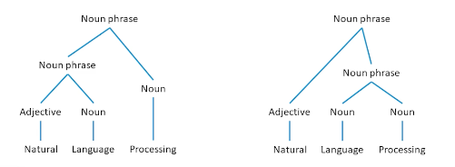
The left tree in the means the processing of natural languages which is exactly what we want computers to be able to do. Now let’s take the exact same phrase, but to put language and processing together into a noun phase, and add adjective to that, now I have language processing, which is natural, which is what humans do but does the exact opposite of what we want computers to do.

Other examples:

We saw the woman with the sandwich wrapped in paper
- What was wrapped in paper? The sandwich or woman?
There is a bird in the cage that likes to talk
Miners refuse to work after death.

Probability and statistics

Brief relationship:

Two important mathematical and algorithmic tools. The first way is to use probability and statistics. why?

Take for example these two statement about movie reviews, are they positive or negative?

This film doesn’t care about cleverness, wit, or any other kind of intelligent humor
There are slow and repetitive, but it has just enough spice to keep it interesting.

We can recast this as a probability statement; what is the probability that the review is positive?

$Prob(positive\_review \lvert w_1, w_2, …, w_n)$
$Prob(positive\_review \lvert \text{“there”,”are”,”slow”, “and”, “repetitive”, “parts”})$
What is the probability that we see the word “repetitive” in a positive review?

We can do the same about text generation, e.g

Once upon a time _____
$P(w_n \lvert w_1, w_2, …, w_{n-1})$

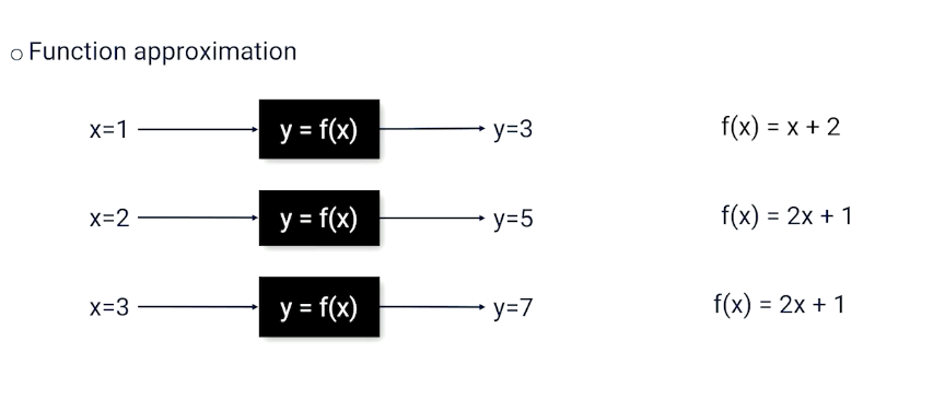
The other tool we have is deep learning.

A significant portion of the state of the art in NLP is achieve using a technique called deep learning
a class of machine learning algorithms that use chains of differentiable core modules to learn from data a function that maps inputs to outputs $f(x) \rightarrow y$
Sentiment classification
- $x$ = input words
- $y$ = positive, negative labels
Text generation, $x$ is input words, $y$ is successor word.
words are everywhere – dialogue, document analysis, document retrieval, etc. Needs to be able to process natural language.
Human languages, which are easy for us, make communication non-trivial for computers

Module 2: Foundations

Random Variables

A placeholder for something we care about.

Random variables can hold particular values
- BEARD <True, False>
- Car <Sedan, coupe,suv, pickup, van>
- Temperature <-100, … + 100>
- Word <a,an, … zoology>

A random variable comes with probability distribution over values. e.g

P(Beard) = <0.6, 0.4>

Likewise for temperature, it can be a continuous so it will be a curve. For words the probability will very sparse.

In NLP, What is the probability that i am in a world in which X has a particular value? What is the probability that I or my AI system is in a world in which some variable X has a particular value?

Do note the notations, $P(X=x) = 0.6$ represents the probability of $X=x$, versus $P(X)$ which is asking for distribution.

Complex Queries

Marginal: $P(A) = \sum_b P(A \lvert B=b)$
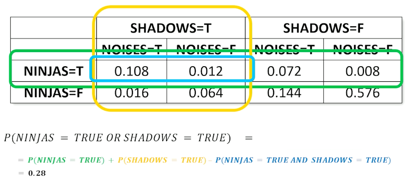
Union: $P(A \cup B) = P(A) + P(B) - P(A \cap B)$
Conditional: $P(A \lvert B) =\frac{P(A \cap B)}{P(B)}$

Full Joint distribution

When you have more than one random variable, the full joint distribution describes the possible worlds.

P(NINJAS,SHADOWS, NOISES) is a full joint distribution

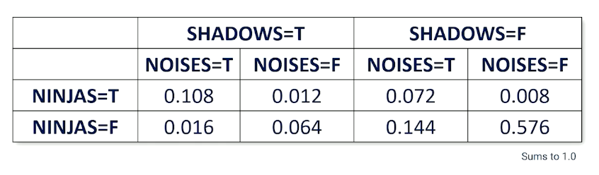
So from the table, about 0.576 of the time, there are no ninjas, no shadows nad noises but also 0.008 where there is a ninja without making any noise and no shadows. So there are a total of $2^3=8$ worlds and note that the probabilities must sum up to one.

So once you have this table, then it is very easy to compute any distributions by looking up. If you are only interested in subset cases, e.g ninja and shadow, then you can do so by summing up marginally.

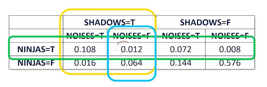
For example the green box is the sum where ninja is present.

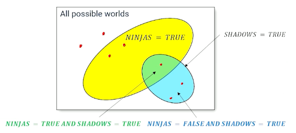
Likewise for another case where you want to know where ninjas or shadows exist:

Again, random variables are things that we care about and want our AI systems to account for. We don’t know the value of the random variables but we know the probability of seeing each possible value. We can compute the probability of any combination of values for a set of random variables (probability of being in different possible words). Sometimes we know how some probabilities will change in response to other variables, called conditional probabilities.

Conditional Probabilities

We are more likely to care about the probability of value of a random variable GIVEN something else is believed to be true.

What is the probability of ninjas given I see shadows?

So e.g $P(ninja \lvert shadows) = \frac{P(ninja \cap shadows)}{P(shadows)}$

Generally, we refer to such things as $P(Y \lvert E = e)$ where $e$ denotes the evidence while $Y$ is the query.

\[\begin{aligned} P(Y=y \lvert E=e) &= \frac{P(Y=y \cap E=e)}{P(E=e)} \\ &= \alpha P(Y=y, E=e) \end{aligned}\]

Under normal literature, $\frac{1}{P(E=e)}$ is called the normalization constant $\alpha$. This has to do with the marginalization of probabilities.

Hidden Variables

Conditional probability query doesn’t always reference all variables in the full joint distribution.

For example,consider $P(Y=y \lvert E=e)$, then if there are more than 2 variables, $P(Y=y \lvert E=e)$ is a partial joint distribution. We can convert it to a full distribution as follows:

\[P(Y=y \lvert E=e) = \alpha \sum_{x \in H} P(Y=y, E=e, H=x)\]

In other words, iterate over all possible H (hidden) values.

Note that you can doit multiple times:

\[P(Y=y \lvert E=e) = \alpha \sum_{x_2 \in H_2} \sum_{x_1 \in H_1} P(Y=y, E=e, H=x, H_1 = x_1, H_2=x_2)\]

Variable Independence And Product Rule

This is to serve as an introduction to bayesian networks.

Two random variables A and B are independent if any of the following are true:

$P(A \lvert B) = P(A)$
$P(B \lvert A) = P(B)$
$P(A,B) = P(A)P(B)$

Product rule allows us to change any joint distribution between variables and turn it into a conditional probability.

\[\begin{aligned} P(A=a,B=b) &= P(A=a \lvert B=b) P(B=b) \\ &= P(B=b \lvert A = a) P(A=a) \\ \end{aligned}\]

And using the equation above, gives us the bayes rule.

\[\begin{aligned} P(A =a \lvert B=b) &= \frac{P(B=b \lvert A=a)P(A=a)}{P(B=b)} \\ &= \alpha P(B=b \lvert A=a)P(A=a) \end{aligned}\]

Bayes Rule With Multiple Evidence Variables

What if I have multiple evidence variables $e_1, e_2$

\[\begin{aligned} P(Y=y \lvert E_1,=e_1, E_2 = e_2) &= \alpha P(E_2 = e_2 \lvert Y=y,E_1=e_1)P(Y=y , E_1 = e_1) \\ &= \alpha P(E_2 = e_2 \lvert Y=y,E_1=e_1) P(E_1 = e_1 \lvert Y=y) P(y=y) \end{aligned}\]

The first step is making use of bayes rule, while the second step is making use of product rule.

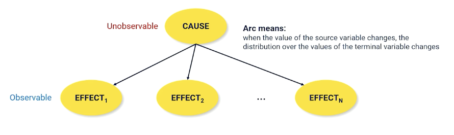
Bayes is particularly useful because we are going to run into lots and lots of situations out in the real world where we often have something called a cause and effect between random variables.

A lot of problems have the form $P(CAUSE \lvert EFFECT)$

The cause is usually something that is unobservable, so I want to know what has caused something that I cannot directly observe given that it has some effect on the world that I can observe.

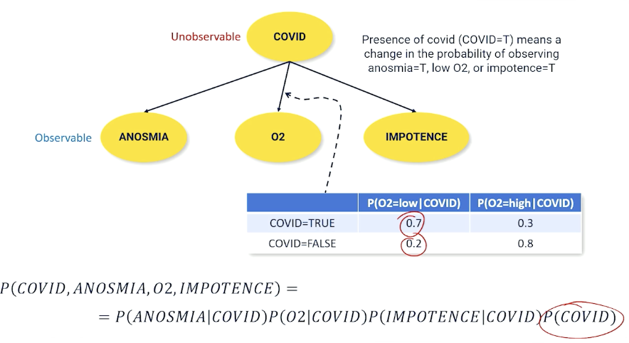
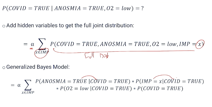
To give an example, such as medical diagnosis $P(COVID \lvert ANOSMIA)$, what is the probability that someone has covid given some of the effects of covid. Anosmia is the loss of smell. To rephrase, how do we detect someone has covid without testing, can we estimate it based on something that is easy to observe?

\[P(Covid = true \lvert Anosmia = True) = \alpha P(A = True \lvert C = True) P(C = True)\]

The interesting bit is when the effects are independent, then we arrive at the generalized bayes model:

\[P(Cause|E_1,...,E_n) = \alpha P(Cause)P(E_1 \lvert Cause)P(E_2 |Cause) \cdots P(E_n \lvert cause)\]

There is the naive bayes assumption, that effect variables are always independent or their casual effects are small to be negligible.

Language Example

Given a target word $W_T$, if we find out the probability whether it exists in a sentence of words $w_1, …, w_n$, then:

\[P(W_T = 1 \lvert w_1,...,w_n) = P(W_T=1)\prod_i^n P(w_i | W_T = 1)\]

Bayesian networks

Bayesian network is just a way of visualizing the casual relationship between random variables. Recall that the cause is usually unobservable - the one we care about but cannot directly observe.

nodes are connected when they have a conditional non independent relationship. So each of effect variables is conditioned on the cause and each of the effects have no edges denoting they are independent.

\[P(X_1, X_2, ...) = \prod_i^N P(X_i \lvert Parents(X_i))\]

You don’t ever have the full joint distribution, but:
You must have a conditional probability distribution for each arc in the bayes net.

Example:

What if we have a missing variables? then we can use the hidden variables:

Documents Are Probabilistic Word Emissions

Another example using movie sentiment instead:

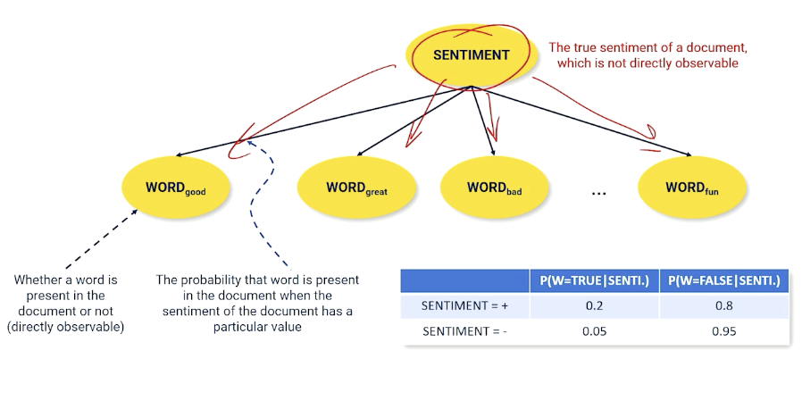
Imagine we have a document, it has an underlying sentiment, and what is doing is spitting out words. If I have a positive sentiment, I am going to spit out more words like good, great, fun etc, and spit out fewer words like bad into this document, and vice versa.

So, whether the word is present in the document which is something directly observable is conditioned on what the underlying unobservable sentiment of that document.

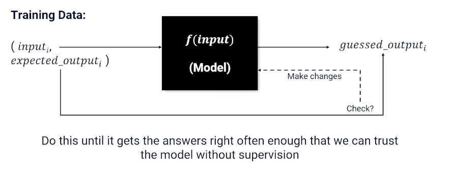
Supervised Learning

Mainly a review of Neural Networks and Deep learning as well as supervised learning.

Supervised learning is to learn a function from a training set of data consisting of pairs of inputs and expected outputs.

Neural Network And Nodes

Mainly talking about nodes representing the gating function, and edges represented weight. The gating function is also known as the activation function such as :

sigmoid $\sigma(x) = \frac{1}{1+e^{-x}}$
Tanh
reLU

Gradient Descent

Remember how to update each weights can be done by gradient descent, which is dependent on the loss function, and ideally we have 0 loss.

Example of loss functions (the are others but lecturer did not mention them):

MSE : $(y-\hat{y})^2$

So we can see how the weights will affect the loss and use the gradient to update the weights to minimize our loss. The steps is skipped but just know that the gradient of each weight is a function of the incoming activation values and the weight applied to each incoming activation value, applied recursively.

\[\begin{aligned} \frac{\partial L(target_k, output_k)}{\partial w} &= \frac{\partial L(target_k, \sigma (in_k))}{\partial w} \\ &= \frac{\partial L(target_k, \sigma (\sum_j w_{jk}out_j))}{\partial w} \\ &= \frac{\partial (target_k - \sigma (\sum_j w_{jk}out_j))^2}{\partial w} \end{aligned}\]

(Feel free to study back propagation yourself).

In summary:

Neural Networks are function approximators
Supervised Learning: given examples and expected responses
Need to know how to measure the error/loss of a learning system
The weights of neural network combined with loss create a landscape
Gradient descent: Move each weight such that overall loss is going downhill
Each weight adjustment can be computed separately allowing for parallelization using GPU(s)

Modern Deep Learning Libraries

There are other libraries like keras, tensorflow and pytorch. This course is going to focus on pytorch.

Neural network is a collection of “modules”
Each module is a layer that store weights and activations (if any)
Each module knows how to update its own weights (if any)
Modules keep track of who passes it information (called a chain)
Each module knows how to distribute loss to child modules
Pytorch supports parallelization on GPUs

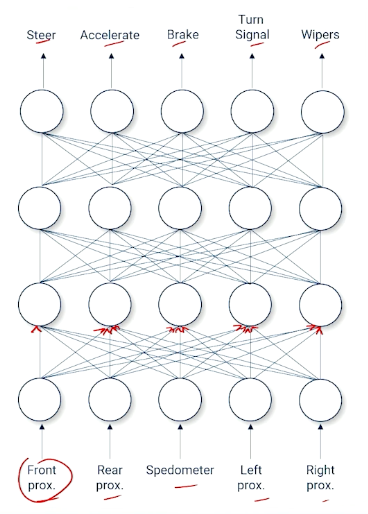
Example of a neural network broken down into layers:

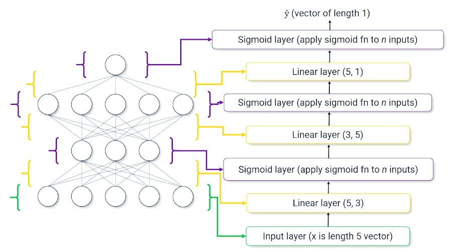
Pytorch Model Example

Note that we have init to define the layers (in the above image),and we can define how the layers are link with the forward method.

  


class BatClassifier(nn.Module):
  def __init__(self):
    self.linear1=nn.Linear(5,3)
    self.sig2=nn.Sigmoid()
    self.linear3=nn.Linear(3,5)
    self.sig4=nn.Sigmoid()
    self.linear5=nn.Linear(5,1)
    self.sig6=nn.Sigmoid()
  def forward(self,x):
    inter1 = self.linear1(x)
    inter2 = self.sig2(inter1)
    inter3 = self.linear3(inter2)
    inter4 = self.sig4(inter3)
    inter5 = self.linear(inter4)
    y_hat = self.sig6(inter5)
    return y_hat

# To predict
model = BatClassifier()
y_hat = model(x)

In pseudo code for training the model, we just need to define the loss function and call backward().

# To train
model = BatClassifier()
foreach x,y in data:
  y_hat = model(x)
  loss = LossFn(y_hat,y)
  loss.backwards()

Pytorch and other modern deep learning APIs make it easy to create and train neural networks
Getting the data is often the bottleneck
Specific design of the neural network can be somewhat of a black art
Pytorch can push data and computations to GPUs, allowing for parallel processing, which can greatly speed up training
Parallelization is one of the reasons why neural networks are favored function approximators.

Module 3: Classification

Introduction to Classification

Examples of classifications: Bayesian, Binary, Multinomial classification. It is important to understand classification because many topics in NLP can be considered as a classification problem.

Document topics (news, politics, sports)
Sentiment classification
Spam detection
Text complexity
Language / dialect detection
Toxicity detection
Multiple-choice question answering
Language generation

Features of classification

Inputs	Outputs
word, sentence, paragraph, document	a label from a finite set of labels

Classification is a mapping from $V^* \rightarrow \mathcal{L}$
- $V$ is the input vocabulary, a set of words
- $V^*$ is the set of all sequence of words
$X$ is a random variable of inputs, such that each value of $X$ is from $V^*$.
- X can take on the value of all possible text sequences
$Y$ is a random variable of outputs taken from $\ell \in \mathcal{L}$
$P(X,Y)$ is the true distribution of labeled texts
- The joint probability wit hall possible text document and all possible labels
$P(Y)$ is the distribution of labels
- irrespective of documents, how frequently we would see each label

The problem is we don’t typically know $P(X,Y)$ or $P(Y)$ except by data.

Human experts label some data
Feed data to a supervised machine learning algorithm that approximates the function $classify: V^* \rightarrow \mathcal{L}$
Did it work? Apply $\textit{classify}$ for some proportion of data that is withheld for testing

An additional source of problem is $V^*$ is generally considered unstructured.

Supervised learning likes structured inputs, which we call features ($\phi$)
Features are what the algorithm is allowed to see and know about
In a perfect world, we simply throw away all unnecessary parts of an input and keep the useful stuff.
- However, we don’t always know what is useful
- But we often have some insight - feature engineering; have a way of breaking down the unstructured data to be something more useful.

Bag of words

In bag of words,

Features are word presence
Discard word order
$\phi$ = { a , the, acting, great, good, plot, …}
- When these words are alone, we call them unigrams, and in pairs will be bigrams, trigrams and so on.
$x$ is a d-dimensional vector of Features
Bag of words can also be word frequency instead of word presence. e.g $\phi_{the} = 2, \phi_{was} = 2$
Other definitions are possible as well.

With that,

A feature vector $\phi(x) \in \mathbb{R}^d$
- Example = $[1, 2, 2, 1, 1, 0, 0, 1, \cdots, 0]$
Every input $x$ is a point in $d$-dimensional space

So if you imagine if every document can be represented in 2 dimensional space, then document can be represented as a vector based on its features:

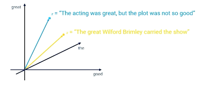
Then we can start to do things like classifications, similarity etc.

Features are what we select for an algorithm to operate on
Good feature sets lead to good algorithm performance.
Bad feature set leads to degraded algorithm performance

Bayesian Classification

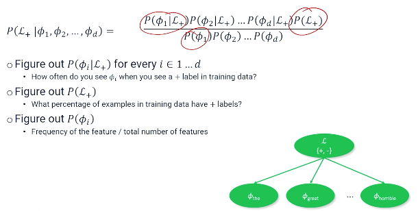
Probabilistic approach to guessing the label that accompanies a text (sentence, document), an example as follows where we are trying to find the label or the sentiment of the document:

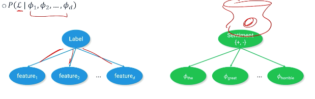
Apply The Bayes equation:

\[P(\mathcal{L}\lvert \phi_1,\phi_2,\phi_3,...,\phi_d) = \frac{P(\phi_1,\phi_2, ..., \phi_d \lvert \mathcal{L}) P(\mathcal{L})}{P(\phi_1,\phi_2,...,\phi_d)}\]

But this equation is very complicated, we can apply the naive bayes assumption - words features are independent of each other:

\[\frac{P(\phi_1 \lvert \mathcal{L})P(\phi_2 \lvert \mathcal{L})...P(\phi_d \lvert \mathcal{L})P(\mathcal{L})}{P(\phi_1)P(\phi_2)...P(\phi_d)}\]

An example:

Can you can also do the same for the negative label:

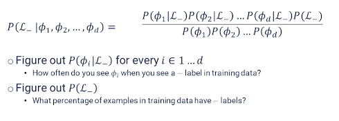
Ultimately, we still need to turn these probabilities into a classification. One way is to see whether:

\[P(\mathcal{L+}\lvert \phi_1,\phi_2,\phi_3,...,\phi_d) > P(\mathcal{L-}\lvert \phi_1,\phi_2,\phi_3,...,\phi_d)\]

We can set $\alpha = \frac{1}{P(\phi_1)P(\phi_2)…P(\phi_d)}$ to ignore the denominator which makes things easier to compute (and also often safe to ignore the denominator in NLP).

In summary:

Bayesian model sees text as a latent (unobservable) phenomenon that emits observable features.
The frequency of which these observable features appear in the text is evidence for the label.
Learning the bayesian model means filling in the probability distributions from the co-occurrence of features and labels.
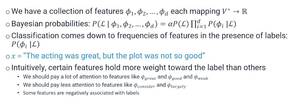
If unigrams don’t give good results, try bigrams or trigrams.

However these comes with limitations; we might want to apply some ML in the future where some of these features are really important to the classification and be able to assign particular weights to those features, possibly even negative weights to say these things might be statistically related to a particular label but actually generally want to think of them as harmful to a particular classification. So the ability to have negative features instead of just every feature being positive with a low or high probability.

Log Probabilities And Smoothing

Two problems:

Multiplying probabilities makes numbers very small very fast and eventually floating point precision becomes a problem.
sometimes probabilities are zero and multiplying zero against other probabilities makes everything zero.

To manage the first problem: shift to log scale. For instance, $log(1)=0, log(0) = -\infty$. Now we do not have to worry about numbers zeroing out (through small probabilities can become very large).

Also, changing to log scale now, we sum things up instead of multiplying them.

$P(A)P(B) \rightarrow = log P(A) + log P(B)$
$\prod P(\phi_i) = sum P(\phi_i)$
$\frac{P(A)}{P(B)} = log P(A) - log P(B)$

For the second problems, zeros can still appear. Suppose “cheese” is a feature but never appears in a positive review, then the conditional probability will be 0 irregardless of the features values ; which also affects our normalization constant $\alpha$.

To solve this, modify the equation so that we never encounter features with zero probability by “pretending” that there is a non zero count of text by adding 1 to the numerator and denominator:

\[P_{smooth} (\phi_i) = \frac{1+count(\phi_i)}{1+\sum count(\phi_i)}\]

We call this technique “smoothing”, naturally this introduces a small amount of error, but it usually does not affect the classification outcome because the error is applied uniformly across all features.

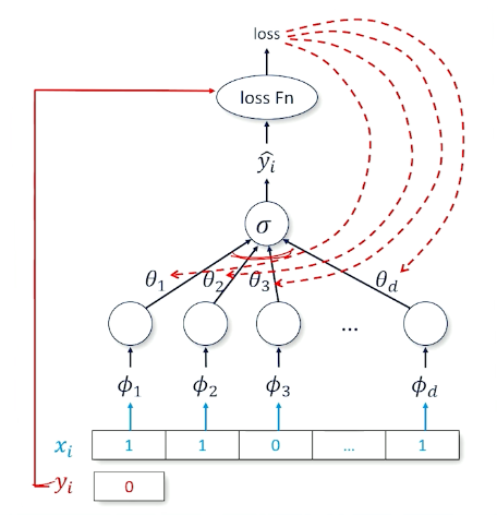
Binary Logistic Regression

A small recap:

In logistic regression, we have a set of coefficients:

$\theta_1, …, \theta_d, \theta_i \in \mathbb{R}$
Also called weights or parameters
If you set the coefficients just right, you can design a system that gets classification correct for a majority of inputs.
But you need to learn them.

On top of this, you need:

Binary labels $\mathcal{L}$
A scoring function $score(x; \theta) = \sum \theta_j \phi_j(x)$
- This can be re-written in matrix form: $ \mathbf{\theta^T \phi}(x)$
Then we can have $classify(x) = sign(score(x;\theta))$

How to learn the weights?

Probabilistically $P(Y=+1 \lvert X = x; \theta) = f(score(x;\theta))$
$f$ converts score into a probability distribution $[0,1]$
An example of $f =\sigma$ the sigmoid function (aka logistic function)
So the sigmoid will return a +1 or -1 whether it is less than 0.5 (or any cut off)

Parameter Learning

Learn the optimal set of parameters $\theta^*$ such that the score function produces the correct classification for every input $x$:

\[\begin{aligned} \theta^* &= \underset{\theta \in \mathbb{R}^d}{argmax} \prod_{i=1}^n P(y=y \lvert X=x_i ; \theta) \\ \theta^* &= \underset{\theta \in \mathbb{R}^d}{argmax} \sum_{i=1}^n log P(y=y \lvert X=x_i ; \theta) \\ \theta^* &= \underset{\theta \in \mathbb{R}^d}{argmin} \sum_{i=1}^n - log P(y=y \lvert X=x_i ; \theta) \\ \end{aligned}\]

Recall that $P(Y=y \lvert X=x ; \theta) = \sigma(y\cdot score(x;\theta))$ and $\sigma = (1+e^{-x})^{-1}$

\[\begin{aligned} \theta^* &= \underset{\theta \in \mathbb{R}^d}{argmin} \sum_{i=1}^n - log \sigma(y\cdot score(x_i;\theta)) \\ \theta^* &= \underset{\theta \in \mathbb{R}^d}{argmin} \sum_{i=1}^n log (1+exp(-y_i \cdot score(x_i ;\theta))) \\ \theta^* &= \underset{\theta \in \mathbb{R}^d}{argmin} \sum_{i=1}^n log (1+exp(-y_i \cdot \mathbf{\theta^T \phi}(x_i))) \\ \end{aligned}\]

Parameter Learning With Neural Networks

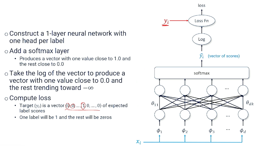
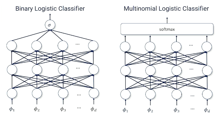
Consider the case of a 1 layer neural network:

Sigmoid at the head to produce a probability close to 1 or close to 0
Target is ${0,1}$ instead of ${-1,1}$

Recall $loss(\hat{y},y) = log(\sigma(y\cdot \hat{y}))$
Multiplies the score $(\hat{y})$ by target $y=\pm 1$ before sending it through sigmoid then log
So, to start thinking about this we are going to use another tool box called binary cross entropy which ia standard loss function:

\[loss (\hat{y},y) = -[y \cdot log(p(\hat{y})) + (1-y) \cdot log ( 1- p(\hat{y}))]\]

Cross entropy means when when y is true, you want $log(p(\hat{y}))$ to be high and vice versa.

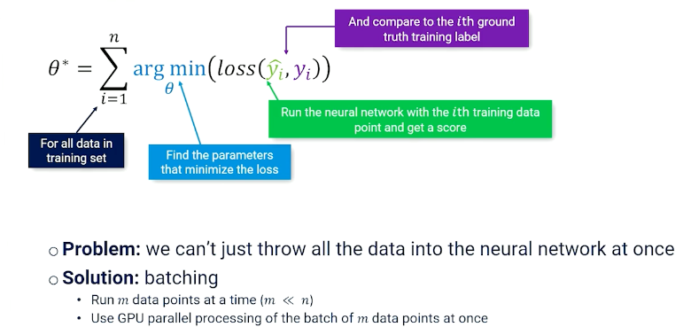
The last thing to talk about is batching, which is just splitting up the data and loading it.

Training

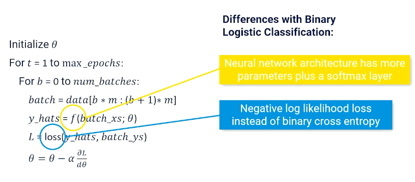
So the entire training looks like this:

initialize θ
For t = 1 to max_epochs:
 For b = 0 to num_batches:
  batch = data[b*m:(b+1)*m]
  y_hats = f(batch_xs; θ)
  L = loss(y_hats, batch_ys)
  θ =  θ - α(∂L/∂θ)

Note that $\alpha$ refers to the learning rate which is usually a hyperparameter, too low and not learn anything and too high you “overshoot” and not converge.

Multinomial Logistic Classification

Suppose we have more than 2 labels, $k$ labels $\mathcal{L} = {\ell_1, …, \ell_k}$

Set of features $f_j : V^* \times \mathcal{L} \rightarrow \mathbb{R}$
$k \times d$ input-output parameters
- $k$ is the number of labels
- $d$ is the number of features
for document $x$ with label $y$, iterate through all labels and all features and set $f_{\ell, \phi}(x,y)$ if feature $\phi$ and label $\ell$ are in the document
What we have:
- A set of $k$ labels $\ell_1, …, \ell_k$
- A collection of $m$ input-output features $f_1(x,y),…,f_m(x,y)$
- Parameters for every input-output features $\theta_1,…,\theta_m$

\[score(x,y;\theta) = \sum_i^m \theta_i f_i(x,y) classify(x;\theta) =\underset{y\in \mathcal{L}}{argmax}(score(x,y;\theta))\]

We are going to want to turn the score into probability
Previously we have used sigmoid $\sigma$
But sigmoid only works for a single comparision, so, what can we do?

Softmax

Need a new tool that can take arbitrary many inputs : Softmax
Softmax takes a vector of numbers and makes one close to 1 and the rest closes to 0, with the vector summing up to 1

\[softmax(x_i) = \frac{e^{x_i}}{\sum_j e^{x_j}} = \alpha e^{x_i}\]

Exponential to make big numbers really big and small numbers really small

Multinomial Logistic Classification As Probability

We want a probability distribution over labels in a document

\[P(Y \lvert X=x ; \theta) = softmax([score(x,y_1;\theta),...,score(x,y_n;\theta)])\]

And one of this numbers will nbe close to 1 and the rest are going to be close to 0.

If we are interested in a specific label, then we can simply calculate $P(Y = \ell \lvert X=x;\theta)$

\[\begin{aligned} P(Y=\ell \lvert X = x ; \theta) &= \frac{e^{score(x,\ell ; \theta)}}{\sum_{\ell'}e^{score(x,\ell' ; \theta)}} \\ &= \frac{e^{score(x,\ell ; \theta)}}{z(x;\theta)} \end{aligned}\]

$z(x;\theta)$ is what makes multinomial logistic regression computationally expensive - to compute the probability even for a single label, you need to calculate / sum across all labels and normalize.

Multinomial Logistic Classification: Parameter Learning

We start from the same equation as before,

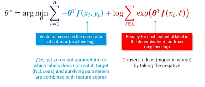
\[\begin{aligned} \theta^* &= \underset{\theta}{argmin} \sum_{i=1}^n - log P(y=y \lvert X=x_i ; \theta) \\ \theta^* &= \underset{\theta}{argmin} \sum_{i=1}^n - log \bigg[ \frac{exp(score(x,y_i ; \theta))}{z(x;\theta)} \bigg] \\ \theta^* &= \underset{\theta}{argmin} \sum_{i=1}^n - log (exp(score(x,y_i ; \theta))) + log {z(x;\theta)} \\ \theta^* &= \underset{\theta}{argmin} \sum_{i=1}^n - score(x,y_i ; \theta) + log {z(x;\theta)} \\ \end{aligned}\]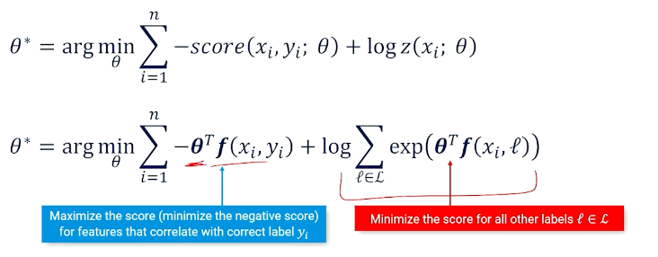

Find the parameters that push up the score for the correct label but push down the score for all other labels
Otherwise, one can just win by making parameters $\infty$

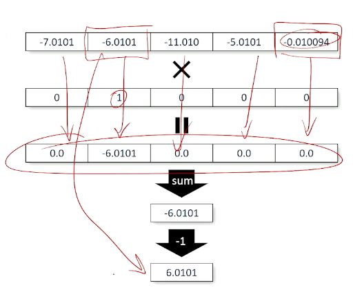
So, the output is a vector of predicted log scores, and vector of target values, and we can multiply them together:

In summary, this is also known as the negative log likelihood loss, so we can have the predicted log scores, vector of target values and we can multiply them divided by the sum, and taking the negative:

Multinomial Logistic Classification: Neural Net Training

The same as before:

So now the $f$ is more complicated and the loss is the negative log likelihood.

Note, in typicals APIs the cross entropy loss module combines the softmax, log and negative log loss together.

Example in pytorch for cross entropy loss

Multilayer Classification Networks

More layers in a neural network can approximate more complex functions. So you can still take the binary logistic classifier or multiple classifications and add more layers.

So this also opens up/allow more sophisticated neural network architectures such as LSTM, Transformers etc.

Module 4: Language Modeling

Language Modeling

A simplified (yet useful) approximation of the complex phenomenon of language production. To recall the use cases:

Autocomplete
Summarization
Translation
Spelling and grammar correction
Text generation
Chatbots
Speech recognition
Image captioning

What makes a good language model?

model fluency of a sequence of words, not every aspect of language production
Fluent: Looks like accurate language (for the purposes of this topic)
Does a sequence of words look like what we expect from fluent language?
Can we choose words to put in a sequence such that it looks like fluent language?

Modeling Fluency

The question becomes, how do we model fluency? Consider the following:

A set of words that our system knows $\mathcal{V}$
How many words does a system needs to know?
- Example: English has $> 600,000$ words
May want to limit that to the top 50,000 most frequently used words
What if we come across a word that is not in the dictionary?
Add special symbols to the dictionary to handle out-of-vocabulary words
- UNK: an unknown word (sometimes also OOV)
Other special symbols:
- SOS: Start of sequence
- EOS: End of sequence

So how can we make use of all these to start modeling? We can resort back to probability:

What is the probability that a sequence of words $w_1, …, w_n$ would occur in a corpus of text produced by fluent language users?
Fluency can be approximated by probability, e.g $P(w_1,…,w_n)$
Let’s create a bunch of random variables $W_1,…,W_n$ such that each variable $W_i$ can take on the value of a word in vocabulary $\mathcal{V}$

Modeling Fluency Examples

Recall the chain rule from bayesian statistics:

\[P(W_1=w_1,...,W_n = w_n) = \prod_{t=1}^n P(W_t = w_t \lvert W_1=w_1,...,W_{t-1}=w_{t-1})\]

The conditional part is the “history” of the t-th words (also called the “context”).

One of the challenges we will face is figuring out how to squeeze the history/context into a representation that makes an algorithm better at predicting the t+1 word. For an arbitrary long sequence, it can be intractable to have a large (or infinite) number of random variables.

Must limit the history/context by creating a fixed window of previous words

How?

First model is to throw away the history completely (unigram approach)
We assume all words are independent of all other words, i.e
- $\prod P(W_t = w_t)$
Obviously wrong

Consider the bigram approach:

Assume a word is only dependent on the immediately previous word:
- $\prod P(W_t = w_t \lvert W_{t-1}=w_{t-1})$
We can extend this to look behind $$ words.

We are not going to make k random variables and try to learn a joint probability across all variables. Instead, we are going to try to approximate the conditional probability using a neural network.

\[P(W_1=w_1,...,W_{n-1} = w_{n-1},W_{n} = w_{n}) = \prod_{t=1}^n P(W_t = w_t \lvert W_1=w_1,...,W_{t-1}=w_{t-1} ; \theta)\]

Can we go a little further? Can we go all the back to one and not be limited by $k$? I.e can our neural network do it in n-gram where n is the length of every sequence in the document? Then we will have a powerful model.

Neural Language Models

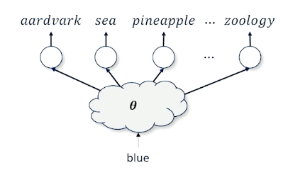
We want to take a word blue and figure out what is the next best word.

The issues is there are 50,000 words
We also have to deal with the context (words before blue)

There are also other problems:

Network networks require inputs to be real-valued numbers
- One possible solution is to use the one-hot vector

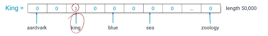
A Token is the index of a word (e.g in the above image, king =2)

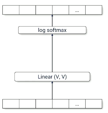
Here is a bigram model, using the one hot vector as input, takes in a single word, and output a single word:

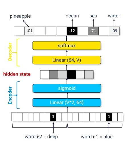
Consider a trigram model it will look like this:

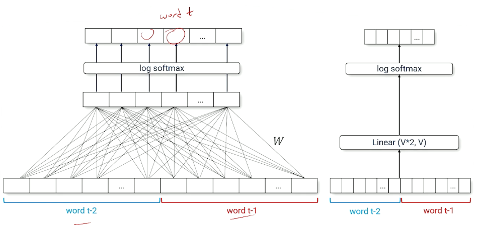
Notice that the linear layer is now $\mathcal{V}*2$, and does not “scale” well.

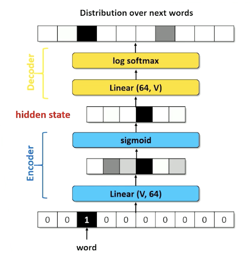
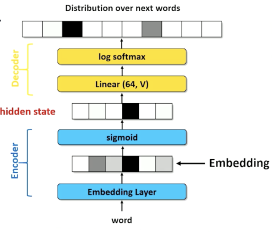
Encoders and Decoders

Ultimately, we need a way to deal with context and history size. Introducing encoders and Decoders

encoder Send input through a smaller-than-necessary layer to force the neural network to find a small set of parameters that produced intermediate activations that approximates the output

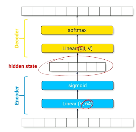
The above image shows the encoder, which is forcing the input layer to be represented by a layer of size 64.
- A good set of parameters will represent the input with a minimum amount of corruption
- Can be “uncompressed” to produce a prediction over the full range of outputs
decoder : A set of parameters that recovers information to produce the output

Now,

Consider a neural network that implements the identity function
Neural network is forced to make compromise
“KING” produces a hidden state activation similar to “regent”

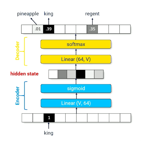
There will definitely be some information loss, and, what is the use of going through such material? We can change the network such that it outputs the next word instead:

The hidden state now compresses multiple words into a fixed size vector
can be reinterpreted as summarizing the history (context vector) - Used interchangeably

Extra note about pytorch, there is a the pytorch.nn.Embedding(vocab_size, hidden_size) that:

Takes a token id (integer) as an input
Converts to a one hot vector of length vocab_size,
maps a vector of length hidden_size.

Encoders perform compression, which forces compromises which forces generalization. We know we have a good compressor (encoder) if we can successfully decompress. However there are still problems:

We cannot have different architectures with different size of context history, like one for bigram, trigram etc. That is not going to work.
With very large scale, its hard to deal with hard long complicated sequences.

Solution? RNN!

Recurrent Neural Networks

Really want one architecture that can manage all these cases.

Text sequences can have different history lengths
Recurrence: process each time-slice recursively

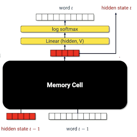
The idea is to use the hidden state and use it back as an input.

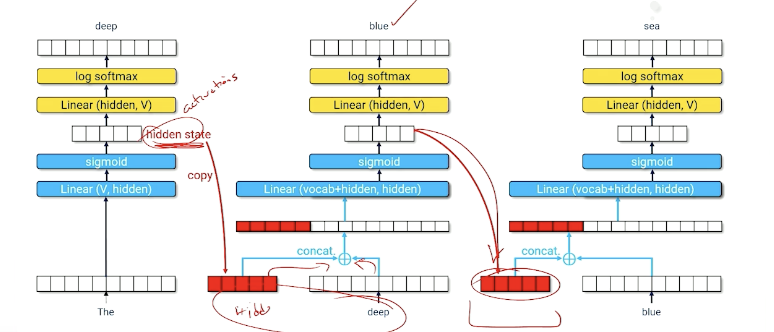
Or to represent it in another form:

Hidden state encodes useful information about everything that has come before
Neural net must learn how to compress hidden state $t-1$ and word $t-1$ into a useful new hidden state that produces a good guess about word $t$.

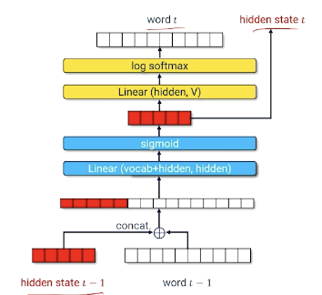
Training An RNN

Training data:
- $x$ token id of $word_{t-1}$
- $y$ token id of $word_t$
Input: $x + \text{hidden state}_{t-1}$
Output: $ \langle log P(w_1), …, log P(w_{\lvert \mathcal{V}\lvert}) \rangle$
Cross entropy loss
- loss = - loss $P(w_1)$
- So if our loss is 0, means our model mostly got it correct, and otherwise.

So, once you have trained the network, how do you start prediction?

Start with a word $(word_i)$ and an empty hidden state (all zeros)
Generate a distribution: $ \langle log P(w_1), …, log P(w_{\lvert \mathcal{V}\lvert}) \rangle$
$word_{t+1}$ is the argmax of the distribution (i.e the one with the highest score/probability)
Feed the output back into the neural network for the next time slice $t+1$.
- In other words use generated word $w_{t+1}$, plus the new hidden state as input to produce word $w_{t+2}$
Repeat until you are done

Now, what else can we do to improve the generation of the neural network?

Generative Sampling

The problem with argmax is it can sometimes results in a local maximum, such as some words always having high scores. Instead of argmax, we can do multinomial sampling from $\langle P(w_1),…,P(w_{\lvert \mathcal{v} \lvert}) \rangle$. We can pick a position/score based on how strong that probability distribution is.

For example:

History = A dark and stormy, what comes next?
So suppose you output words with [(night,0.4), (sea, 0.1), …]
- You will pick night with 0.4, sea with 0.1, and so on.
- This works if your prediction is nice and peak around certain words
However, sometimes multinomial sampling can appear too random, especially when there are alot of options with similar probabilities.
- Can we “train” the neural network to be more “peaky”? E.g instead of $[0.1,0.1,0.1,…]$ we want $[0.8, 0.01,…]$

To achieve this, we can introduce a new variable called temperature, $T \in (0,1]$ and sample from:

\[norm \bigg(\bigg\langle \frac{log P(w_1)}{T}, ..., \frac{log P(w_{\lvert \mathcal{v} \lvert})}{T}\bigg\rangle\bigg)\]

Divide every probability score by this temperature value, and then normalize this so it is between 0 and 1. Let’s observe what will happen:

Divide by $T=1$ means the distribution is unchanged
Dividing by a number $T <1$ means all the numbers increase
as temperature goes to 0, the highest score goes to infinity.
- This will look / act more like argmax.

However, RNN can still make mistakes as generation from a RNN is an iterative process of feeding outputs into the neural network as inputs. RNNs tend to forget parts of context-hard to pack things into the context vector.

So, LSTM!

Long Short-Term Memory Networks

Hard to learn how to pack information into a fixed-length hidden state vector
Every time slice the RNN might re-use part of the vector, overwriting or corrupting previous information.

An example (The vector here represents an embedding):

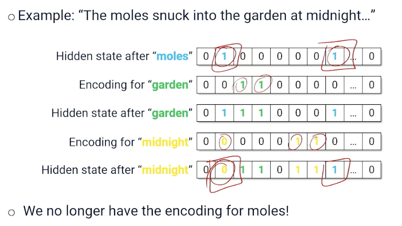
If you notice, the hidden state after midnight has overwritten a piece of information here so that we can capture midnight; so both midnight and moles need to use index 1; we effectively lose the information about moles.

That brings us to LSTM, would be nice if the neural network could learn:

What is worth forgetting
Which part of the new word input is worth saving
This means we can maintain a “better/valid” hidden state longer.

How does Long short Term Memory (LSTM) achieve this?

Replace internal parts of a RNN encoder with a specialized module called a memory cell.

LSTM: A Visual Walkthrough

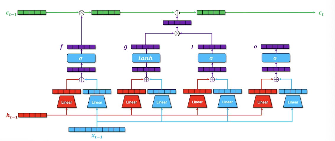
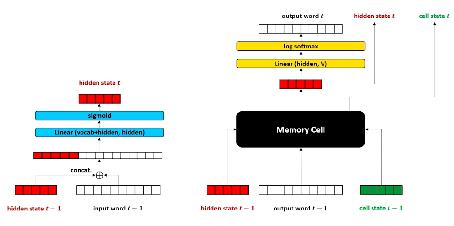
Let’s first look at the computational graph:

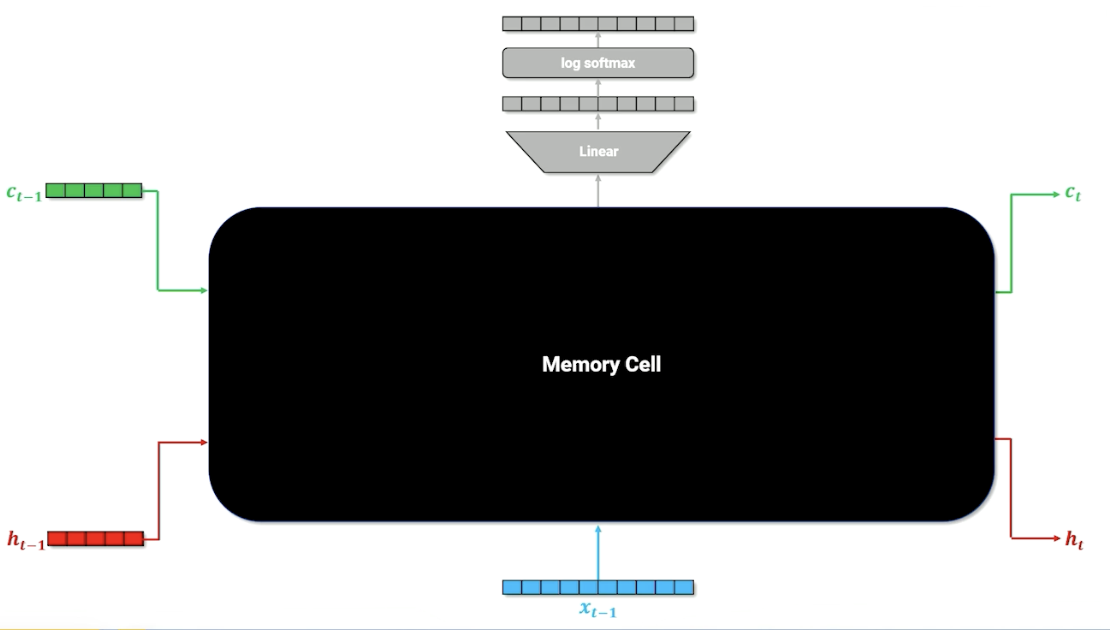
$x$ is the one hot vector of the word, and $h$ is still the context/history, similar with RNN. There are now is an additional parameter $c$, the cell memory. Let’s look deeper into this cell memory (black box) to know what is going on:

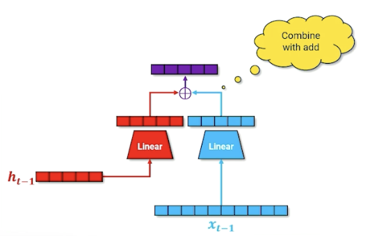
Remember, the linear layer compress the one hot into something useful. We also do the same for the hidden layer and combine them:

Then, we take that and run it through a sigmoid (which will turn some values to 0 or 1). We are going to call this the forget gate.

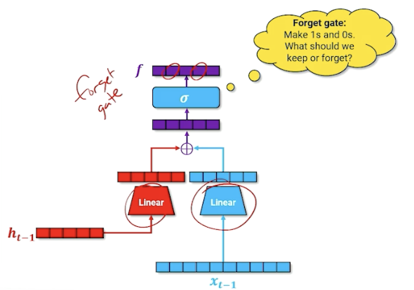
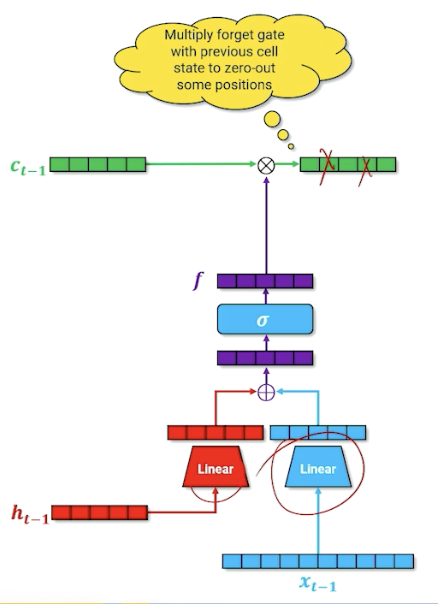
We take the output of the forget gate, and multiply it with the cell memory - think of it as “deleting” information in the cell memory into the next time step; this is how the neural network learns what to forget. (For those familiar, this is the forget gate)

In addition, we are going to do another parallel structure inside or our neural network that is going to do our cell memory update. Note that the linear layers will learn a different set of parameters. (For those familiar, this is part of the input gate)

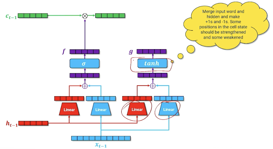
The goal is to produce a new cell memory, we do not use a sigmoid but tanh. To recall, tanh produces numbers that are $[-1,1]$ instead of sigmoid $[0,1]$. So what we are going here is merging our word and our hidden state to try to figure out what things should be $+1, -1$. The way we can interpret this is. this is going to be introduced to our cell memory from the previous state, by saying which input in the cell should be strengthened or weakened by adding/substracting one.

We are not going to add this to the cell memory yet, and going to introduce another parallel structure and have another gate that essentially considers whether this word $x$ should be added to the cell memory. (For those familiar, this is called the input gate). Is this word important that should be carried on or it can be ignored?

We take the input gate $i$ and multiply by the new cell memory $g$:

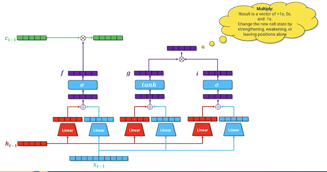
This resulting vector not just has plus ones and negatives one but also zeros, so either strengthen, weaken our cell memory or zero, leaving it unchanged. We finally take this and multiply with $c_{t-1}$ to form the new $c_t$.

For one last time, we have another parallel block (For those familiar, this is the output gate), the idea here is to say what needs to be part of the next hidden state, which is going to be used for both the decoder but it is also going to be passed on to the next layer time step in our recurrence.

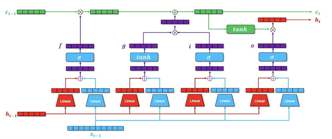
We are also going to incorporate in our cell memory, so if we want to figure out what goes into our hidden state, it is going to be a combination of what we want to go forward through our output state as well as whatever cell memory is going to say. The second tnah here is going to squish everything back down to $[-1,1]$ (Lecture mentioned $[0,1]$ somehow but its tanh? ) and combining it with our output gate to produce our new hidden state.

LSTM: A Mathematical Walkthrough

The forget gate can be written as:

\[f = \sigma(W_{x,f}x + b_{x,f} + W_{h,f}h + b_{h,f})\]

The input gate / cell memory can written as:

\[\begin{aligned} f &= \sigma(W_{x,i}x + b_{x,i} + W_{h,i}h + b_{h,i}) \\ g &= tanh(W_{x,g}x + b_{x,g} + W_{h,g}h + b_{h,g}) \\ \end{aligned}\]

Then update cell state $c$:

\[c_i = (f \times c_{i-1}) + (i \times g)\]

Then, we can now calculate our output gate as well as update our hidden state:

\[\begin{aligned} o &= \sigma(W_{x,o}x + b_{x,o} + W_{h,o}h + b_{h,o}) \\ h_i &= o \times tanh(c_i) \end{aligned}\]

In summary,

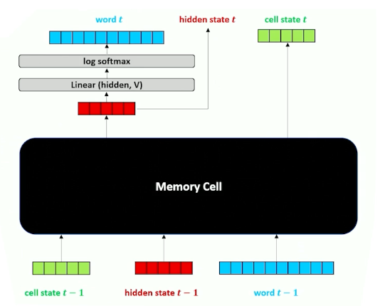
The full LSTM encoder-decoder network containing the memory cell
Hidden state summarizes the history of the text
Cell state is information needed for the memory cell to do its job, passed from time step to time step

As a side note, usually for LSTM, we refer to the entire block as one LSTM block and do not map out the internals of it.

LSTM cells pass extra cell state information that does not try to encode text history but information about how to process that history - meta knowledge about the text history. LSTM were SOTA for a long time and are still useful when handling recurrent data if indeterminate length, and holds “Short-term” memory longer. But LSTM can still get overwhelmed trying to decide what to encode into the context vector as history gets longer and longer.

Sequence-to-Sequence Models

Special class model that is build on top of LSTM. Recall the structure of LSTM:

This is because sometimes data is of the form:

$x_i = SOS\ x_{i,1}, x_{i,2}, …, x_{i,n}\ EOS$
$y_i = SOS\ y_{i,1}, y_{i,2}, …, y_{i,n}\ EOS$
- Each x,y is a sequence of words that are clumped together and are considered a single whole.

The reason why this is a special case is because this comes up very often especially in translation. So translation is usually about converting a phrase (or a sequence) in one language into another language.

Translation also comes with its own problems, such as the phrasing, words not having a one to one mapping, etc. Sometimes we need to look the full sequence to be better informed on our prediction. In order to handle sequence to sequence data:

sweep up an arbitrary input sequence and encode it into a hidden state context vector.
Good for picking up on negations, adjective order, etc. Because the whole input sequence is in the context vector.
Then decode it into an arbitrary length sequence
Stop decoding when EOS is generated

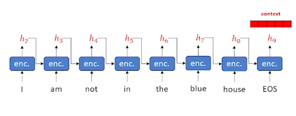
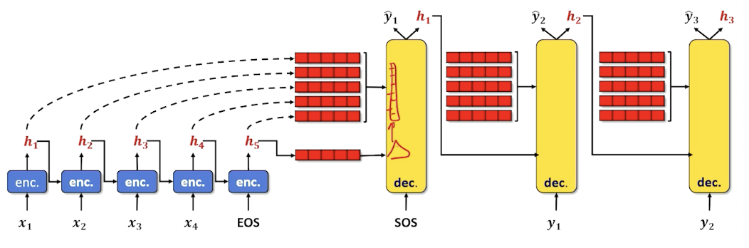
Sequence-to-Sequence Example

Consider the following example where we keep finding words and update our hidden state:

Now, we take that context, and start sending it into the decoder:

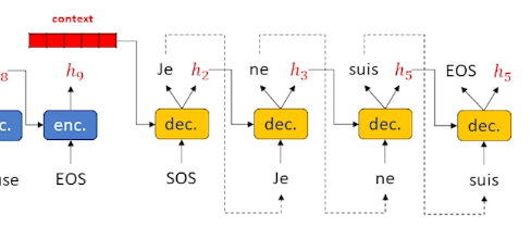
And when we see the EOS tag we can stop.

This is a little different from the previous LSTM where we did it word by word. Essentially, we have taken the decoder and put it to one side. The decoder need some sort of output word (as opposed to an input word) as well as a hidden state that keeps track of what is going on. As a result, we need to put another encoder in the decoder layer, we cannot work directly on words and hidden state. So in a Sequence to sequence, the decoder itself has an encoder inside. The encoder (within the decoder) is usually an LSTM as it works really well, and in most diagrams the cell state is omitted to keep the diagrams clean.

In summary:

Separate the encoder and decoder
Change the decoder to take an output word and hidden
Allow us to do one of the most important things in modern neural language modeling: Attention

Sequence-to-Sequence Model Training

How do we train it when we have a separate encoder and decoder?

Now that it is separate, our training loop is going to have two parts as well. It is going to iterate through the encoder and then it is going to iterate through the encoding.

For the encoder:

Set hidden state $h_0^{enc} = \vec{0}$
Do until $x_j = EOS$
- Encode $x_j$ and $h_j^{enc}$ to get $h_{j+1}^{enc}$
- Increment $j$

For the decoder:

Set $x_0^{dec} = SOS$
Set $h_0^{dec} = h_{j+1}^{enc}$
Do until $\hat{y}_j^{dec} = EOS$ or until we hit max length
- Decode $x_j^{dec}$ and $h_j^{dec}$ to get $\hat{y}_{j+1}^{dec} \text{ and } h_{j+1}^{dec}$
- Set $x_{j+1}^{dec} = \hat{y}_{j+1}^{dec}$
- Because this is training: loss = loss + loss_fn($\hat{y}_{j+1}^{dec}, y_{j+1}$)
- Increment $j$

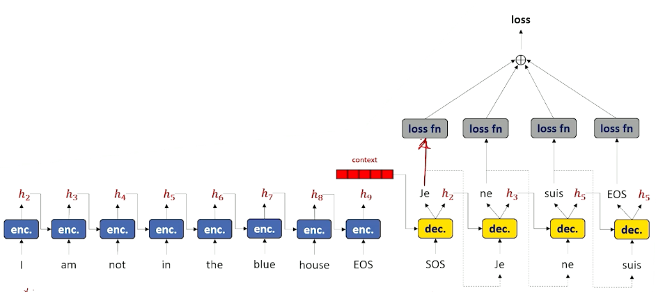
Once we have done all of this, back propagate loss. But this time our loss is the aggregated loss.

Visually we can look at it like this (the loss reflects the entire sequence at once instead of word by word):

Teacher Forcing

We are going to introduce a new trick to make the neural network learn even better, known as teacher forcing.

Instead of using the decoder’s output at time $t$ as the input to the decoder at time $t+1$…
Pretend our decoder gets the output token correct every time.
Use the true training label $y_{i,t}$ as input to the decoder at time $t+1$

So for our decoder, It looks like this instead:

Do until $y_j=EOS$
- Decode $y_j$ and $h_j^{dec}$ to get $\hat{y}_{j+1}^{dec} \text{ and } h_{j+1}^{dec}$
- Set $x_{j+1}^{dec} = y_{j+1}^{dec}$ i.e ignore the prediction and set to the true value
- However, for our loss function, we still use the prediction:
  - loss = loss + loss_fn($\hat{y}_{j+1}^{dec}, y_{j+1}$)
- Increment $j$

So this is good in the sense because in the early phase, our decoder is getting all the words wrong, which compounds the problem - i.e your next word is built on top of a previous wrong word. With teacher forcing, we just use the prediction to compute the loss but use the true word to proceed.

We can get a little more fancy with this:

Can perform teacher forcing some percentage of hte time and feed in decoded tokens the remaining percentage of the time.

In summary:

Teacher forcing makes training more efficient
Sequence to sequence works for data that can be split into discrete input and output sentences:
- translation
- X and Y can be adjacent sentences to learn to generate entire sentences at once

Moving on to attention next - how we cna make sequence to sequence a little bit more intelligent by being smarter about how it looks back at its own encoder in order to help me figure out what to do in specific slices in the decoder step. This will help out with some of the issues with forgetting and overwriting of our context vectors.

Attention, part 1

Finally, Attention is all you need.

Recall that:

Parts of the hidden state are continuously overwritten and can forget
Do we need to throw away all the intermediate hidden states during sequence encoding?
Attention: The decoder to look back through the input and focus a “spotlight” on various points that will be most relevant to making the next prediction of the next output token.
Pull the attended information forward to the next prediction.

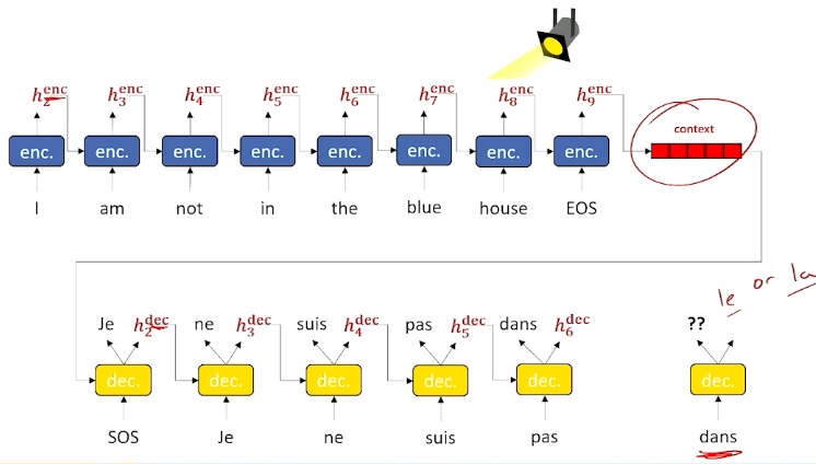
Will be great if at prediction of the next word, to look back / spotlight at the decoder stage to identify what was encoded at that particular time slice and if the network knew that, may be able to bring this encoder information forward and make much better choice.

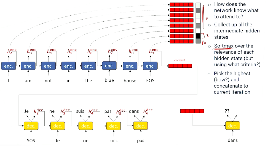
The next question is, how do we know which time slice to look at then? In which section should we pay attention to?

Grab every single encoder output hidden state and save them and stack them up in a big Q.
Decide which is the most important to us, so we have a tool for doing selection - Using softmax!
- But what criteria to use for softmax? We still need to figure this out.
- Assuming we are able to do so, take the best one, and use it as input for the next decoder step.
- And we do this for every step.

Attention, part 2

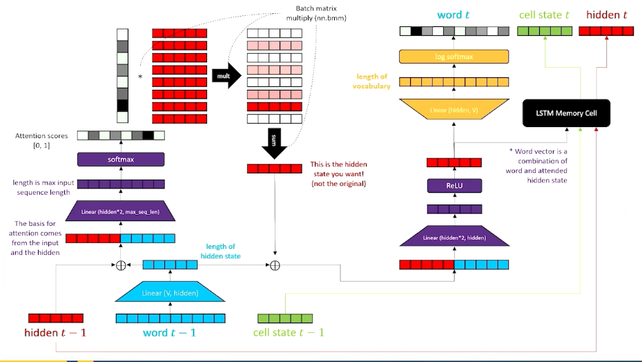
Let’s take a deeper look now - How we get attention to the decoder:

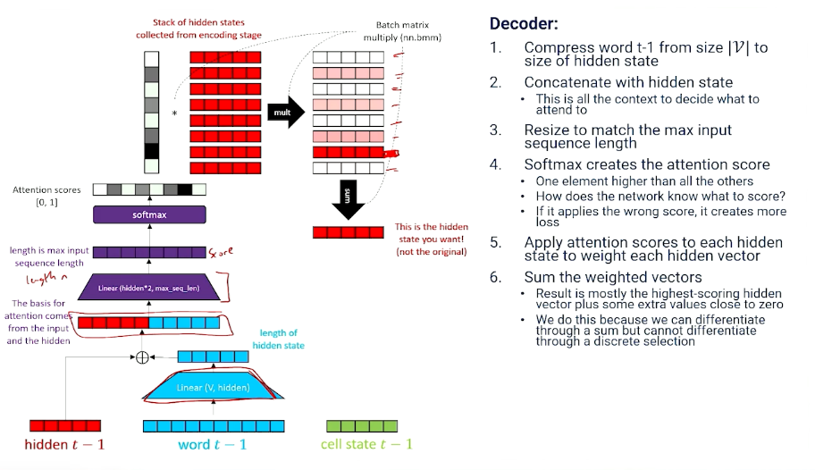
To summarize,

Attention: dot product (inner product) of a softmaxed context vector and a matrix of candidates.
Everything that might be relevant to choosing what to attend is packed into the context vector
Network learns how to generate the attention score with linear transformation.

Now, on to the decoder part (we have only finished the attention portion):

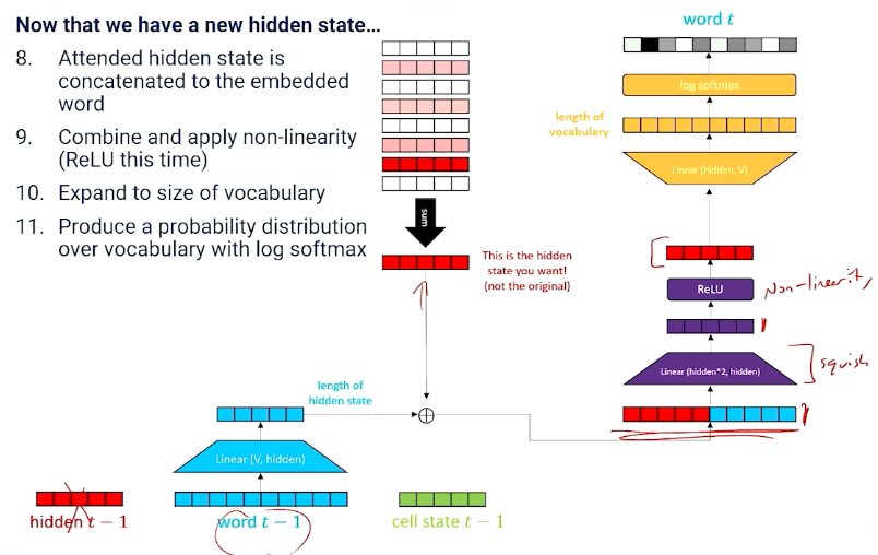
We still need to produce new hidden state and memory cell state!

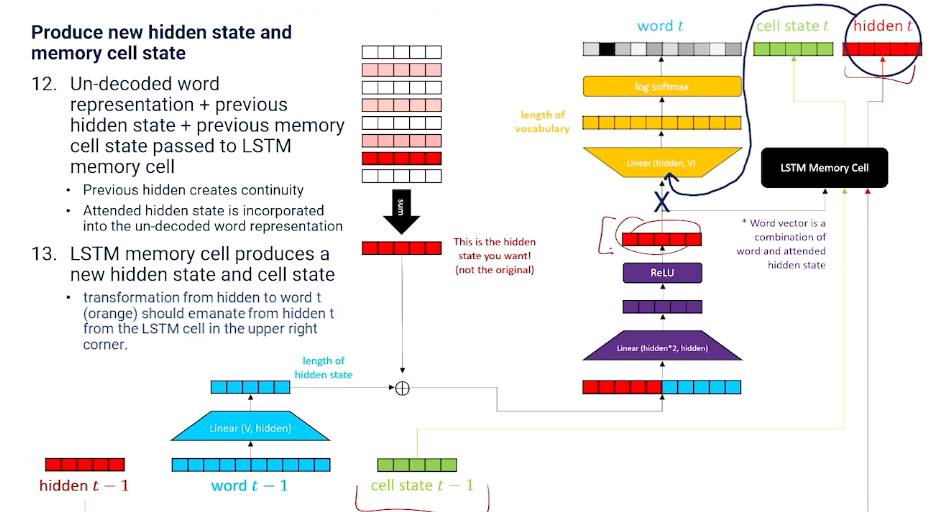
And we do so with a LSTM memory cell layer.

Putting it all together this is what we get:

In summary,

Attention is the mathematical equivalent of “learn to choose from inputs” and is applied in the decoder.
Attention does not require sequence to sequence, it can be applied to a regular LSTM if there is a buffer of previous words and intermediate hidden states to draw on.

Different Token Representations

Taking a slight detour here to talk about token representation.

Up to now we have assumed a token is a word and the vocabulary is a word and the vocabulary is a very large number of words.
vocabulary would be letters $\mathcal{V} = [a,b,c,…,z,1,2,3,… punctuation]$
vocabulary size is small, but the language model has to learn to spell out every word one letter at a time.

There is another way thinking about tokens inbetween having letters and full words, and thats something called subword tokens.

Breakdown complicated words into commonly recurring pieces.
- For example “Tokenize” $\rightarrow$ “token” + “ize”
- vocabulary would contain common words, common word roots, suffixes, prefixes, letters and punctuation
Neural network mostly works on word tokens but occasionally has to learn how to use context to assemble a complex word.
In the worst case, neural network can learn to spell really rare, complex words from letters.
Sub-word vocabulary can cover most of english with fewer tokens ~50,000
One additional advantage: No need for out-of-vocab (UNK) tokens, as handling these is difficult.

Perplexity, part 1

How do we test / evaluate NLP/language models? How do we know when they work well? Even if the loss is low, is it learning what we want it to learn or learning anything useful?

Recall that:

Language models are all about modeling fluency: probability ~ fluency.
\[P(W_1=w_1,...,W_{n-1} = w_{n-1},W_{n} = w_{n}) = \prod_{t=1}^n P(W_t = w_t \lvert W_1=w_1,...,W_{t-1}=w_{t-1} ; \theta)\]
That is: The probability of every word is conditioned on its history

Now, perplexity:

A measure of how “surprised” (perplexed) a model is by an input sequence
A good language model is one that is good at guessing what comes next

Branching factor

Branching factor: number of things that are likely to come next.
If all options are equally likely, then branching factor = number of options
But if different options have different probabilities, then:
- Branching factor = $\frac{1}{P(option)}$
  - Etc flipping a coin where $P(heads) =0.5$, then branching factor is $\frac{1}{0.5}=2$.
  - If $P(heads) = 0.75$ then branching factor is $\frac{1}{0.75}=1.33$.

Coming back:

The probability of a word differs given its history $P(w_t \lvert w_1, …, w_{t-1})$
So the branching factor will be $\frac{1}{P(w_t \lvert w_1, …, w_{t-1})}$
The more plausible alternatives, the more likely the model will make the wrong choice.

Ok, but we have introduced a new problem, consider:

Probability of a sequence of words (or the probability of this sentence) is:
\[P(w_1,...,w_n) = \prod_{t=1}^n P(w_t \lvert w_1,...,w_{t-1})\]
But, longer sequences would have a smaller probability - So this makes things unfair as well; longer sequences will likely have a smaller probability
so we need to normalize by length by taking the $n^{th}$ root, which is done by using the geometric mean:
\[P_{norm}(w_1,...,w_n) = \prod_{t=1}^n P(w_t \lvert w_1,...,w_{t-1})^{\frac{1}{n}}\]
And so the branching factor of a sequence of words:
\[\prod_{t=1}^n \frac{1}{P(w_t \lvert w_1,...,w_{t-1})^{\frac{1}{n}}}\]
Perplexity is just the branching factor of a sequence of words:
\[perplexity(w_1,...,w_n) = \prod_{t=1}^n \sqrt[n]{\frac{1}{P(w_t \lvert w_1,...,w_{t-1} ; \theta)}}\]

Perplexity, part 2

Taking the previous equation, and transforming it into log space:

\[\begin{aligned} perplexity(w_1,...,w_n) &= exp\bigg( \sum_t^n log(1) - \frac{1}{n}log P(w_t \lvert w_1, ..., w_{t-1};\theta) \bigg) \\ &= exp\bigg( \sum_t^n - \frac{1}{n}log P(w_t \lvert w_1, ..., w_{t-1};\theta) \bigg) \end{aligned}\]

Perplexity is also the per-word exponentiated, normalized cross entropy summed up together: so now, we have established a relationship between perplexity and loss.

Therefore, in the case of RNN:

Recurrent neural networks generate one time slice at a time
Perplexity is the exponentiated negative log likelihood loss of the neural network:
- $perplexity(w_t) = exp(-log P(w_t \lvert w_1,…,w_{t-1};\theta)) = exp( Loss(\hat{y},target))$

To recap,

Perplexity is loss, the lower the better
Perplexity is how surprised the language model is to see a word in a sentence
More possible branches means model is more likely to take the wrong branch
Perplexity($w_t$) =$x$ means the odds of getting the right token is equivalent to rolling a 1 on an $x$-sided die.
- Example: Perplexity($w_t$) = 45 means the model has a 1/45 chance of getting the right token.
- But if it was 2 then that means it has 1/2 chance of getting the right token.

With that:

During training, we look for loss to go down
During testing (on unseen data), we look for a low perplexity
- The best language models in the world achieve a perplexity of ~20 on internet corpora
Perplexity doesn’t mean non-sense - It means that the model makes a choice other than one that exists in a corpus
- Even if we have a high perplexity, it doesn’t mean only one word is going to make sense and a whole bunch of words are not going to make sense; maybe the top 20 words still make sense or reasonable words, e.g “Why did the chicken cross the road” vs “cross the street”.
  - It is still going to be fluent and we are not going to be necessarily upset. It just wasn’t the one perfect word according to some test set.

Module 5: Semantics

Document Semantics

Semantics: What word and phrase mean
Problem: Neural Networks don’t know what word means
- By extension neural network don’t know what a document is about
- Words are just one-hot vectors

So, How do we represent the meaning of a document?

Multi-hot
- Set a 1 in each position for every word in a document.
- The values are the same but some words are more important than others.
- If you want to figure out if two documents are related to each other you want to rely on words that are effective at distinguishing documents
- Look for ways to determine which words are important

Term Frequency-Inverse Document Frequency

TFIDF - a specific technique trying to decide whether two document are semantically similar to each other without really having the semantics of words and documents themselves.

Give weight to each word based on how important it is

Term frequency : If a word shows up frequently in a document, it must be more important than other words:

\[TF(w,d) = log(1+freq(w,d))\]

$freq(w,d)$ is how many times $w$ appears in document $d$
The log forces the TF to grow very slowly as the frequency of a word gets larger.

Inverse Document Frequency : Words that are common in all documents are not very important

\[IDF(w,D) = log \bigg( \frac{1 + \lvert D \lvert }{1 + count(w,D)}\bigg)+1\]

$ \lvert D \lvert$ is number of documents
$count(w,D)$ is how many documents in $D$ contains $w$
As the count increases, the ratio goes towards 1.

So, TF-IDF:

\[TFIDF(w,d,D) = TF(w,d) \times IDF(w,D)\]

Apply TF-IDF to every word $w$ in every document $d$ to get a vector

In summary:

TF-IDF provides a more nuanced document representation of a document than a multi-hot
Next we look at how to compute document similarity and retrieve the most similar documents

Measuring The Similarity Documents

Document Retrieval: given a word or a phrase (itself a document), compare the query to all other documents and return the most similar.
Given two documents, represented as vectors, how do we know how similar they are?

One way is to use the vector distance:

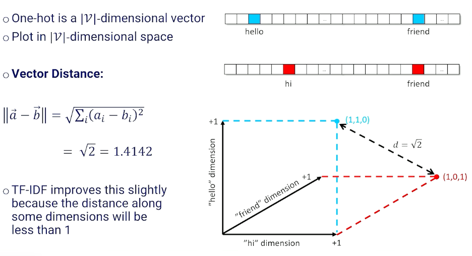
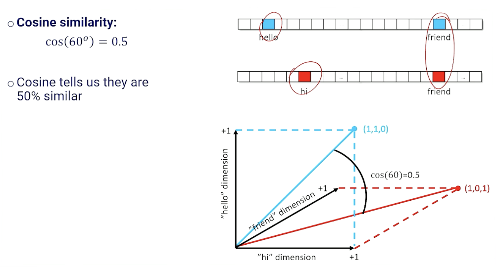
Another way is to use the cosine distance:

Now, on document retrieval:

Create a $1 \times \lvert \mathcal{V} \lvert$ normalized documetn vector for the query($q$)
Create a normalized vector for every document and stack to create a $\lvert \mathcal{D} \lvert \times \lvert \mathcal{V} \lvert$ matrix $\mathcal{M}$.
Matrix multiply to get scores
Normalized the final vector
This is the same as computing the cosine similarity

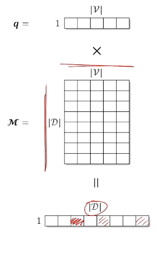
\[cos(\vec{a},\vec{b}) = \frac{\vec{a} \cdot \vec{b}}{\lvert\lvert \vec{a}\lvert\lvert * \lvert\lvert\vec{b}\lvert\lvert}\]

Take the argmax to get the index of the document with the highest score (or get the top-k to return more than one)

There are still two issues:

Require a $\mathcal{V}$ length vector to represent a document
Does not capture the fact that some words are similar (“hi” vs “hello”)

Word Embeddings

The problem with TF-IDF just now is the way we index them in a vector even though they probably mean the same thing.

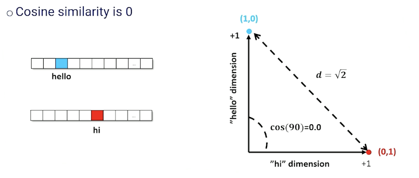
Instead of a $\lvert \mathcal{V} \lvert$ - dimensional space, we want a space that intuitively maps similar words and phrases close to each other. This is also known as embeddings:

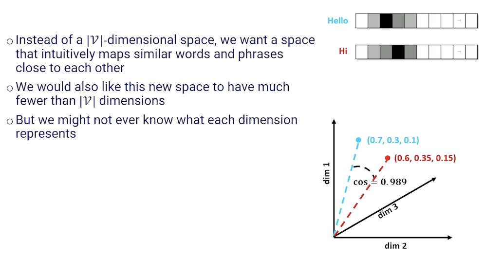
So, how are we going to get these embeddings?

Take a one hot (or multi hot) and reduce it to a $d$ -dimensional space where $d \ll \lvert \mathcal{V} \lvert $
Use a linear layer with $\lvert \mathcal{V} \lvert \times d$ parameters $\mathcal{W}$
- Compress a one-hot into a d-dimensional vector

Why does this work?

One-hot for the $i^{th}$ word selects a set of $d$ weights and all others are zeroed out
These remaining weights are a $d$-dimensional representation of the indexed word
Because we are multiplying by 1s and 0s, the $d$ weights $W_i$ are identical to the $d$-dimensional vector of activations at the next layer up.

Looking at the matrix of weights in the linear layer:

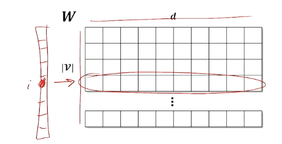
Each row in $W$ is an embedding for each token in vocabulary
One-hot selects the row
Learn weights that capture whatever relationship we need

Word Embeddings Example

Recall the RNN architecture where we have an encoder layer:

We call the lienar compression layer in the encoding the embedding layer:

token to one hot
Linear from length $\lvert \mathcal{V} \lvert$ to $d$ length vector
For simplicity moving forward, we are going to assume we can turn the word directly to an embedding.

Embedding layer in an RNN learns weights of an affine (linear) transformation
Whatever reduces loss in the output probability
- Must have compromises (words having similar activations)
- We hope those compromises map similar words to similar vectors
- Still no guarantee on semantic similarity
Embedding layer is task specific
- Because ultimately it is being fed into a NN with a loss function for a specific task.
Question: can we learn a general set of embedding?

Word2vec

Maybe we don’t need to know what each word means:

Distributional semantics : a word is known by by the company it keeps
Words that man approximately the same thing tend to be surrounded by the same word

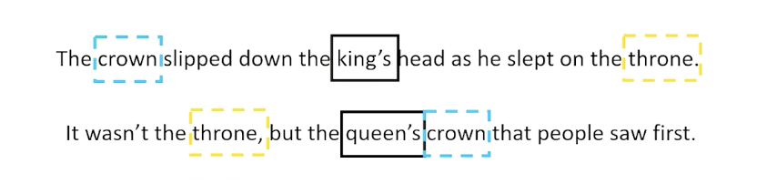
For example we always see king and queen together, maybe they mean something very similar in terms of semantics
Again - the idea is we don’t need to know what the word mean if words with similar meaning have similar embeddings

Then the question is:

How can we train an embedding to use this concept of distributional semantics
Can a word be predicted based on surrounding words?
- The crown was left on the throne when the ???? went to bed at night.
- Probably king or queen is a reasonable choice; although we can’t quite tell which is better
Can we predict the surrounding words based on a single word?

Take out a word in the middle of a sequence and ask a neural network to guess the missing word
Loss is the cross entropy of the probability distribution over words

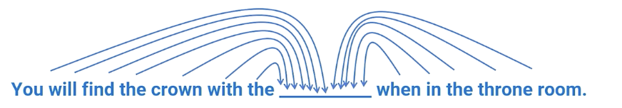
Similarly, we can look at the opposite of the problem:

Can a window of words be predicted based on the word in the middle of the window?

Take a word and guess the words to the left and right
Loss is the cross entropy of each blank given the word in the middle
Break up into skip grams (bigram on non-adjacent tokens)
- E.g given word $w_t$, predict $w_{t-i}, w_{t+1}$ for some $i$.
Predict each skip-gram separately

This is also known as the word2vec approach and there are actually two approaches to word2vec:

continuous bag of words
or skip grams

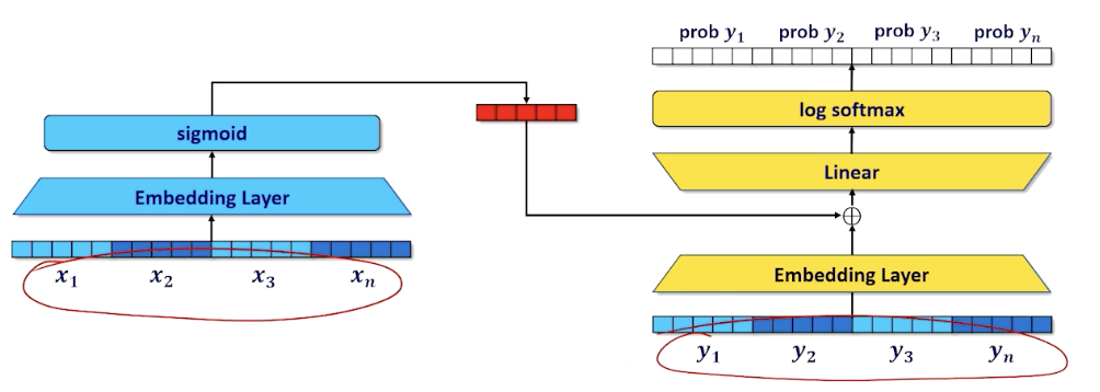
Let’s look at the continuous bag of words (known as CBOW) first, for a window of size $k$, what we are doing is we are taking a particular chunk of document and note that the document is missing a word in the middle.

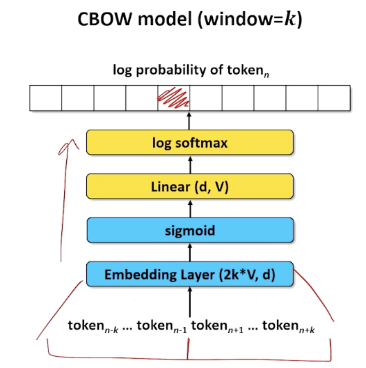
So we take the $2k$ words off the left and right of the target word and asking the neural network to predict the missing word, in this case the embedding layer is $2k*V$ and outputs a/compresses it into $d$ dimension.

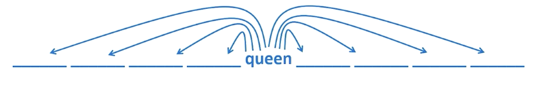
Now, let’s look at the skip gram model which is to look at a particular word and trying to guess the surrounding words

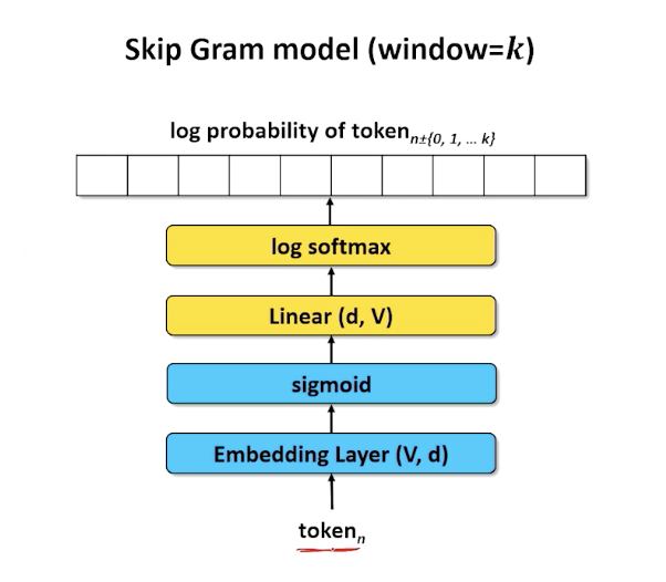
So again, the word will be turn into a dimension of size $d$
Because this is skip gram, we do not really care about the positions of the words but instead look at words with high activations.
- And the k highest activations are the words that are most likely to be in window around our $n^{th}$ word
- Doesn’t need to be a sentence, can be jumbled up - we are just looking for words
Compute the entropy of each of the prediction matches the actual words we would find in a span taken from our actual document.
- The math side of things is omitted which is a little complicated.

Embedding

Let’s see what we can do for our embeddings, remember in either CBOW or skip gram we have the embedding layer

We can extract teh weights from the embedding layer
- Each row is the embedding for a different token in the vocabulary

We can now do something interesting:

such as computing the cosine similarity using the embedding.
- $cos(\vec{v}{queen}, \vec{v})$
We can also do retrieval; find documents that are semantically similar
- Which Wikipedia document is most relevant to “Bank deposit”
  - Chattehoochee river
  - Great Recession of 2017
Can also do analogies - add and subtract word embeddings to compute analogies
- Georgia - California + peaches = ?

Again, to recap - words that represent similar concepts tend to be clustered closely in d-dimensional embedding space.

Vectors can be added and subtracted

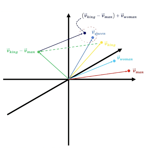
E.g King - man + woman = Queen

Also:

Most points in embedding space are not words
Search for the nearest discrete point

What about document embedding?

Add each word vector
Word vectors pointing in the same direction strengthen the semantic concept

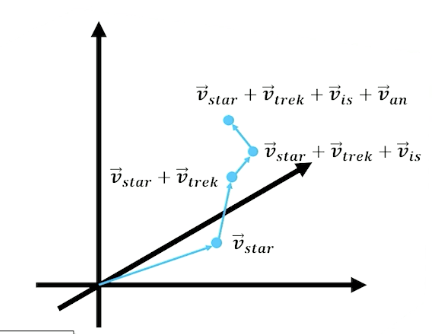
Normalize the resultant vector
- Value of any of the $d$ dimension is the relative strength of that abstract semantic concept
- Necessary for cosine similarity

In summary:

Word2vec is a learned set of word embeddings
- Can either use continuous bag of words (cbow) or skip grams
Word embeddings can be used in word similarity, document similarity, retrieval, analogical reasoning etc
Text generation must learn an embedding that helps it predict the next word, but the embedding linear layer can be seeded with word2vec embeddings
We will find embeddings in just about all neural approaches to natural language processing.

Module 6: Modern Neural Architectures

Introduction to Transformers

Current state of the art, at least in 2023.

Recall that:

RNNs process one time slice at a time, passing the hidden state to the next time slice
LSTMs improved the encoding to the hidden state
Seq2seq collects up hidden states from different time steps and let the decoder choose what to use using attention
- Note how the decoder is side-by-side by the encoder and has it’s own inputs in addition to the hidden state (token from the previous time step)
- $x_s$ are the inputs to encoder, $h_s$ are the outputs
- $y_s$ are the inputs to decoder, $\hat{y}_s$ are outputs
- Loss computed on $\hat{y}_s$

To add:

Recurrent Neural networks, LSTMs, and Seq2seq exists because recurrence means we don’t have to make one really wide neural network with multiple tokens as inputs and outputs.
- The wide model was originally considered a bad idea because:
- inflexible with regard to input and output sequence lengths
- computationally expensive
But sequence lengths is not a big deal if you make $n$ ridiculously long (~1,024 tokens) and just pad one-hots with zeros if the input sequence was shorter.
Computation also got alot better capable of more parallelization
- 2017: First transformer (65M parameters) was train on 8 GPUs for 3.5 days
- 2020: GPT3 Transformer (175B parameters) was trained on 1,024 GPUs for a month

Transformers: Combining 3 Concepts

Introducing transformers - Combine 3 insights/concepts.

First concept: Encoder/Decoder that operates on a large input input window consisting of a sequence of tokens

Entire input and output sequence provided at once
Like Seq2seq the decoder takes a hidden state and entire output sequence, which no longer needs to be generated token by token.

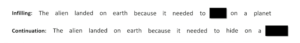
Second concept: Masking

Blacking out tokens so that the network has to guess the missing token
One way is infilling: Guess a word in an arbitrary position in the middle of a sequence
Another way is continuation: Guess the word at the end of the sequence.
Transformers are sometimes called masked language models
Recall: We have seen this in word2vec is a robust way of learning to embed

Third concept: Self-attention

Instead of collecting up hidden states from previous time steps, all time steps are “Flowing” through the network in parallel
Each time step can attend (softmax and dot product) to every other time slice.
As if network has to guess each word - what other words increase the odds of the actual word?

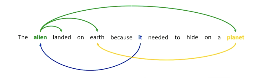
For example, a word like alien might want to attend to words like landed and earth, because alien is involving in the landing and is involved in this entity called earth and earth is the planet. So earth and planet seems to mean the same thing, as well as alien and “it”.

So when we put all of these things together, we are going to have a very large network:

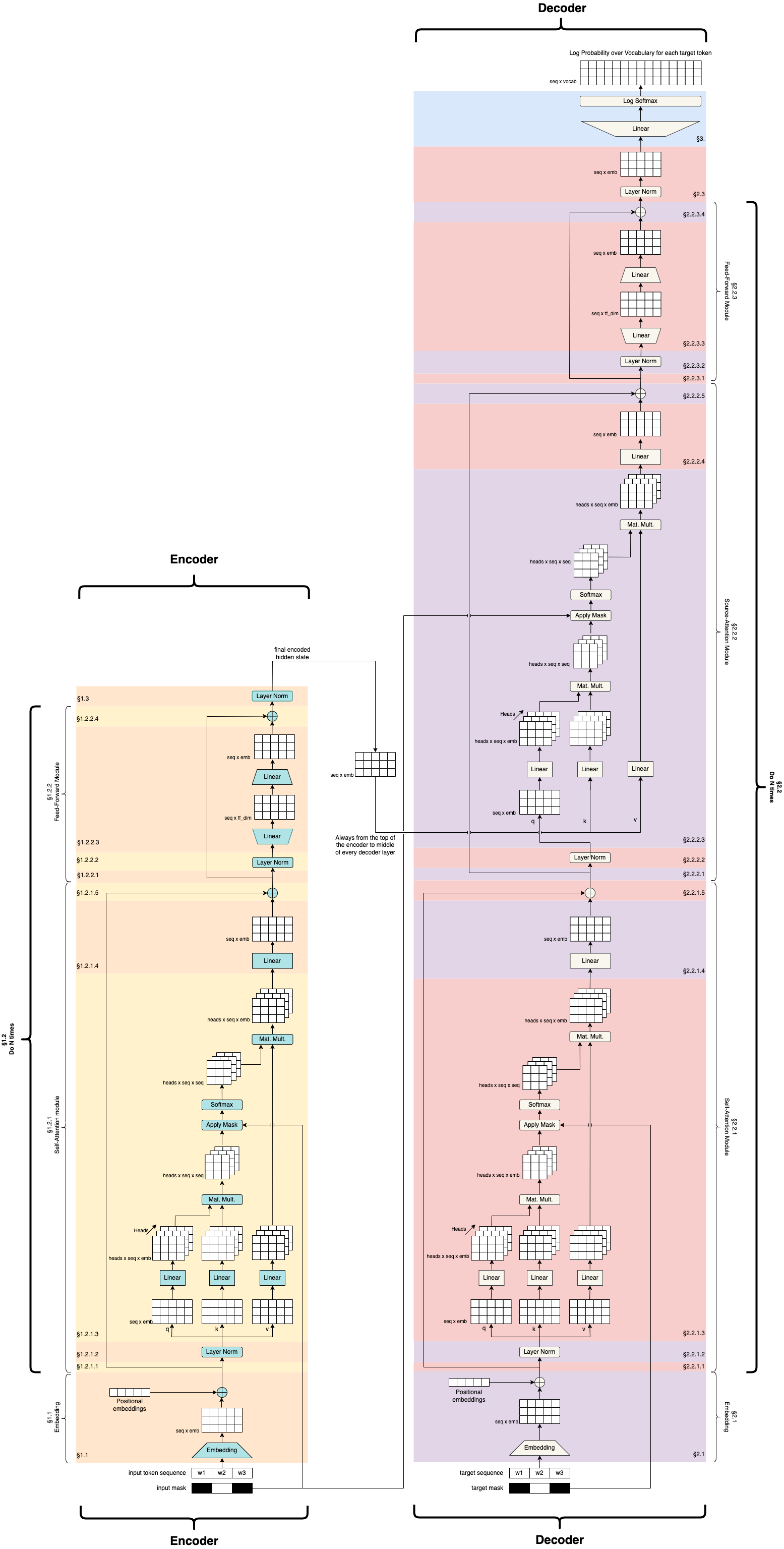Credit: https://github.com/markriedl/transformer-walkthrough

So we have an encoder/decoder situation with encoder and decoder side by side as we are often used to seeing, and then we start to deal with all these concepts of attention and masking and so on.

We will walk through the encoder and decoder, and discuss some note worthy transformer architecture such as BERT and GPT.

Transformer Encoder

The focus here is on self attention inside the encoder - each position in the sequence is able to select and incorporate the embeddings of the most relevant other positions.

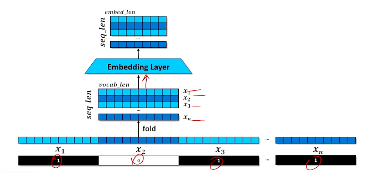
Given a sequence of tokens $x_1,…,x_n$ and a mask (in the above image $x_2$ is masked)
Stack the one-hots to create a matrix
Embed the one-hots into a stack of embeddings

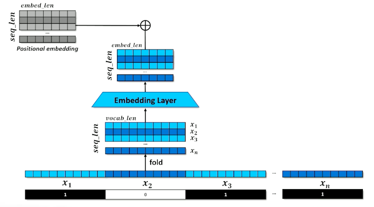
The problem is:

The network doesn’t know what order the tokens came in
Add positional information to each element of each embedding

What is a positional embeddings?

Sine and Cosine functions at different scales
Each embedding get a small number added or subtracted
Identical tokens in different places in the input will look different

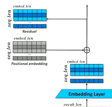
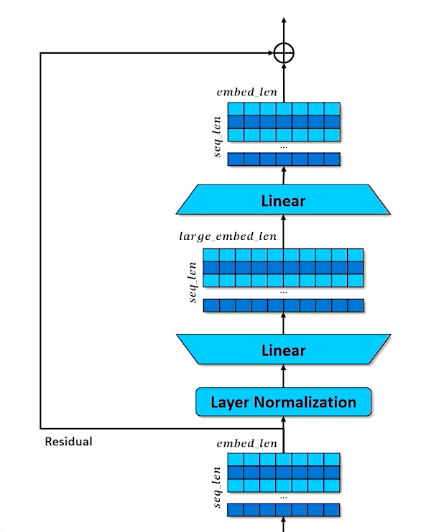
Set aside a residual

A branch in the computational graph
Tensor is untouched on one branch and manipulated on the other branch
The manipulations are then applied to the residual and merged with the residual copy
This will be revisited in the future to understand why we need this residual

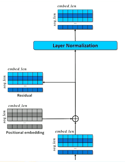
All dimensions of all tokens are made relative to the mean $x’ = \frac{x-mean(x)}{\sigma(x) + \epsilon}$
After normalizing, add trainable parameters $(W,b)$ so that the network can adjust the mean and standard deviation how it needs $x’’ = Wx’ +b$

Transformers: Self-Attention

Self-attention is a mechanism to capture dependencies and relationships within input sequences. It allows the model to identify and weigh the importance of different parts of the input sequence by attending to itself.

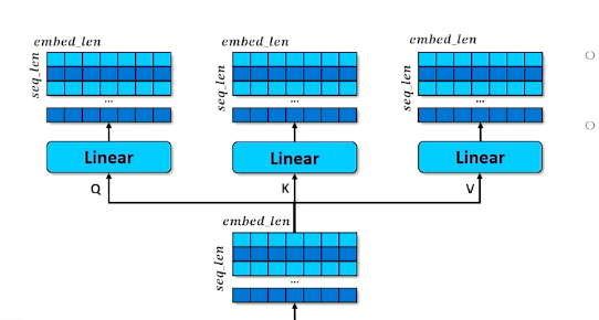
Make three copies of the embeddings
- Don’t over think it, just think of a hash table
A normal hash table matches a query (Q) to a key (K) and retrieves the associated values (V)
Instead, we have a “soft” hash table in which we try to find the best match between a query and a key that gives us the best value
First we apply affine transformation to Q,K and V
Learning happens here - how can Q, K and V be transformed to make the retrieval work best (results in the best hidden state to inform the decoder)

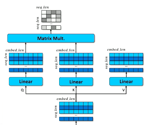
How does a query match against a key?
Multiply Q and K together to get raw scores

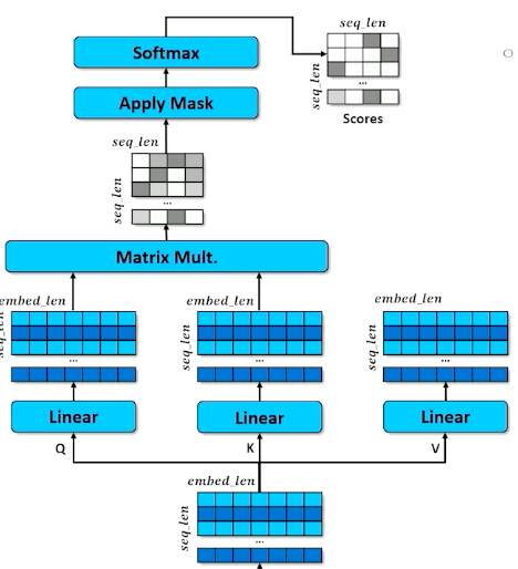
Apply the mask to indicate tokens that cannot be attended to (make numbers in masked rows close to 0)
Apply softmax to “pick” the row each token thinks is most important

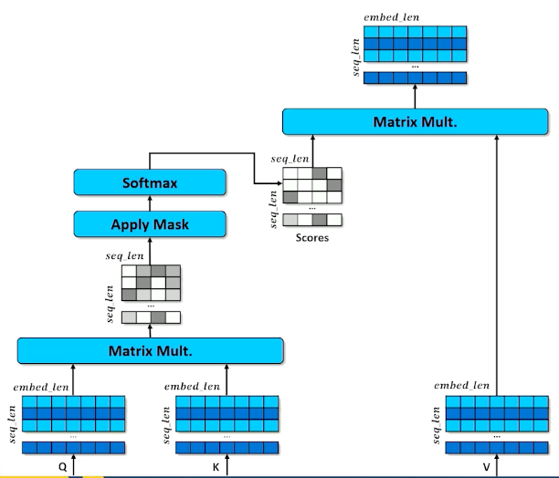
Each cell in the scores matrix indicates how much each position likes each other position
Softmax means each row should have a column close to 1 and the rest close to 0
Multiplying the scores against V means each position (row) in the encoded $x$ grabs a portion of every other row, proportional to score.

Example:

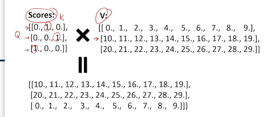
In Q, the softmax is 0/1 for simplicity, in reality they are all probabilities so we will get a little of everything.
So what we can see is it is shuffling/jumbling up the embeddings - the one closest to 1 will preserve the most values.

We will see in the next section how we make use of this “jumbled up” embeddings.

Self-Attention Process: Outputs

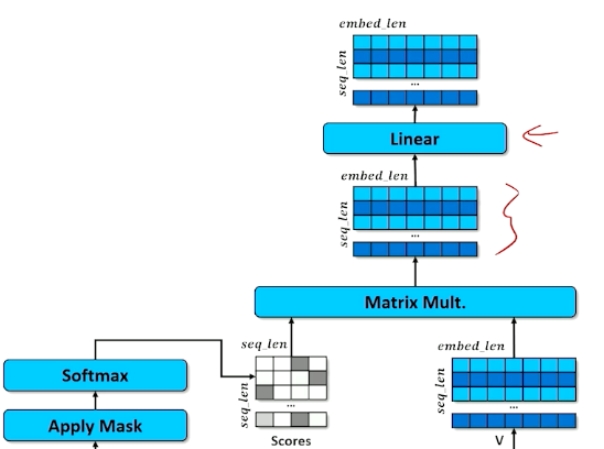
Apply a linear layer learns to do whatever is necessary to make this jumbled up set of embeddings to the next stage. (Instructor says whenever you are not sure if it is required to alter the weights, just a linear layer )

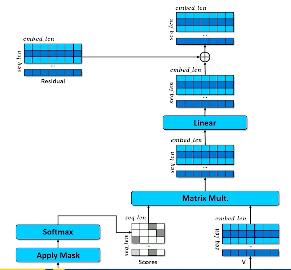
Now, coming back to the residual:

Remember it was a pure copy of the embeddings
Results of the self-attention are added to the residual
Important to retain the original embedding in the original order
reinforce or inhibiting embedding values (according to the transformation just before it)
Now each embedding is some amount of the original embedding as well as some proportion of every other embedding attended to.

Set aside the residual a second time
Layer Normalization
Learn to expand and compress the embeddings
Expansion give capacity to spread concepts out
Compression forces compromises but in a different configuration
Re-apply residual

In summary:

Stack the embed a sequence of $n$ tokens
Split the embedding into query, key, and value and transform them so that Q and K can be combined to select a token from V with softmax
Add the attended-to V to teh residual so that certain token embeddings are reinforced or diminished but never lost
Do steps 2 and 3 $k$ more times to produce a final stack of $n$ hidden states, one for each of the $n$ original tokens

Multi-Headed Self-Attention

One last small detail to our encoder: Multi head

The encoder configuration is single-headed self attention
Each token can attend to one other token
But we might want each token to attend to more than one token to account for different contexts or word senses
Multi-headed attention applies self attention $h$ times

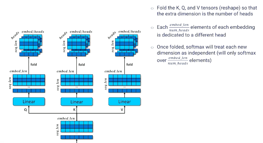
Note that we sacrifice embed_len in this case, but we can simply extend it in the earlier layers if we need to.

Then, we still do the same thing to multiply our Q and K together:

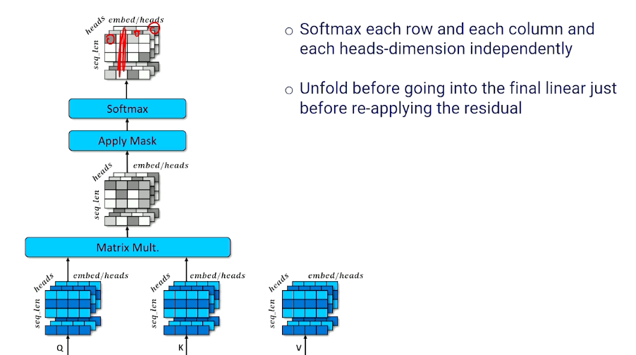
To summarize:

Each token position can select $h$ different token positions
Each $h^{th}$ of each token embedding is a separate embed
When unfolded, each row is now a combination of several other token embeddings
Important because each token may be informed by the presence of several tokens instead of just one other token.

Transformer Decoder

Now, we turn our attention (pun intended) to the decoder side of things which will show us how we made use of the output from the encoder.

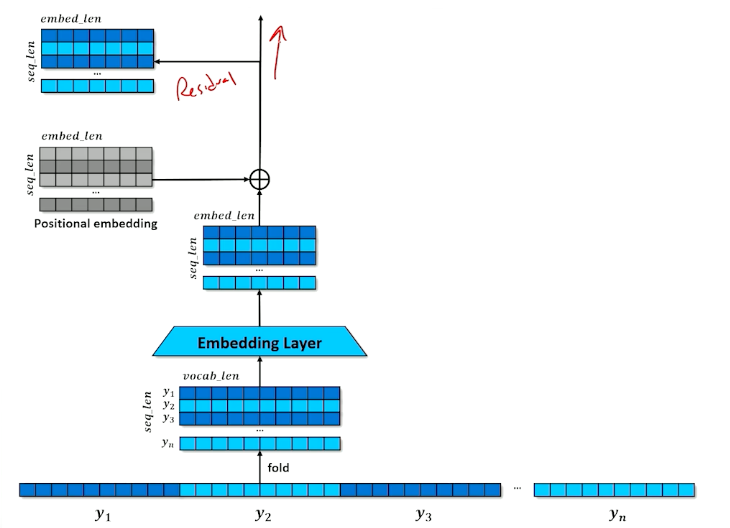
The decoder is almost the same as the encoder
- It still outputs the residuals and store a separate copy
Like Seq2seq, the decoder will take the hidden state from the encoder
It also takes an input the $y$ tokens, as if seq2seq was teacher-forced
The decoder-output will be a log probability distribution over tokens.

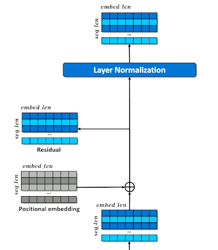
Again, similar steps with the encoder, and this make things ready for self attention again.

The embedded tokens are $Q$
The major difference is now we do not make $K$ and $V$ copies

and instead:

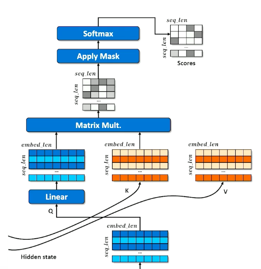
Hidden state from the encoder is copied into $K$ and $V$
Decoder has to learn (linear parameters) how to match the best key to get the right value
Doing so increases the probability of guessing the right output tokens

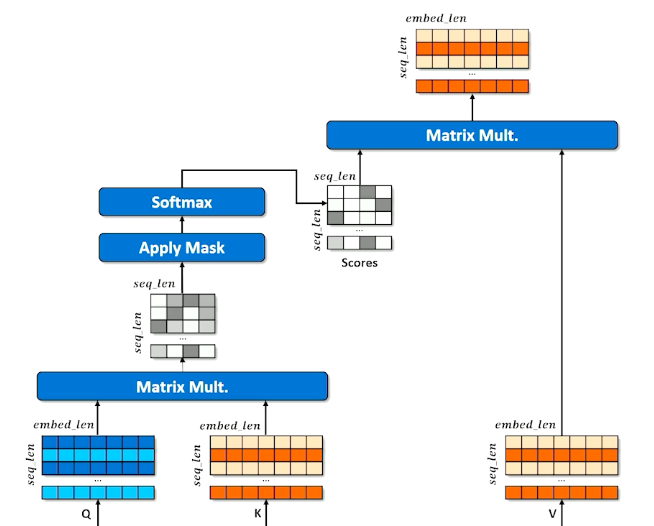
The above diagram shows single headed but we actually do mutli headed

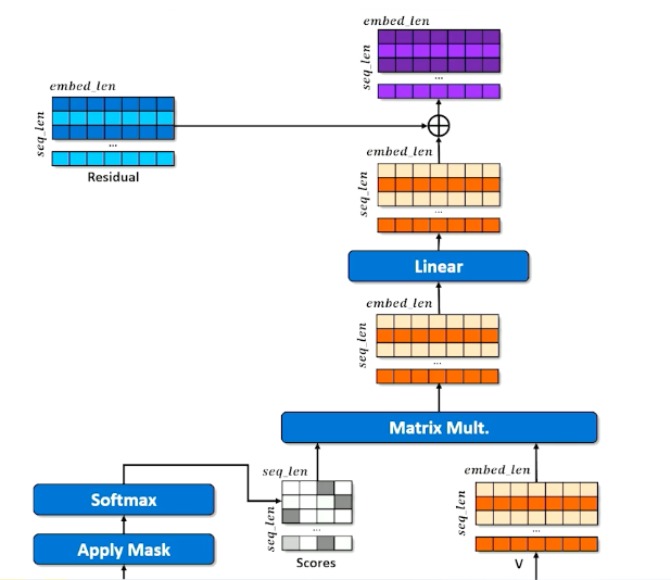
And continue to send up the chain and do some linear transformations
- Also add the residuals that is created during the decoder.

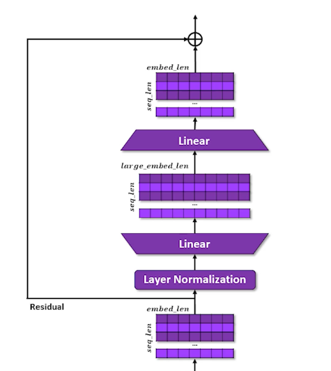
The decoder creates the query to be applied against the key and value from the encoder
Learn to select the most important hidden state from the input
- Do this $n$ times

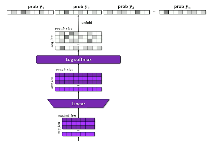
And finally, we have the generator:

basically just the expansion out to the vocabulary / prediction.
Remember here we are interested in the original masked location, so we go back and figure out the masked-out probability distribution (in this case $x_2$)
- Ultimately what we care about from a generation standpoint

For computing loss, we only look at the masked positions(s)

Compute KL-divergence between each predicted token $\hat{y}_{masked}$ and the actual token $y_{masked}$

BERT

Bert stands for Bidirectional Encoder Representation from Transformers

Addresses the need for contextual embeddings
Example:
- The heavy rain caused the river ot overflow its <MASK> and flood the valley.
- The increase in interest rates caused the <MASK> to stop approving loans
- You are probably thinking about the word <Bank> which can mean the financial institution or one side of the river. So how can a language system differentiate between between these two users when the word is exactly the same?
This issue plague many natural language systems prior! Recall:
- Word2Vec makes a word and tries to find an embedding that allows the word to be guessed based on other words around it
- Word2Vec during training would sometimes see water-related words and financial-related words and find an embedding that satisfied both context
- The embedding of a word should be different based on other words around it
And this is what BERT is trying to do:

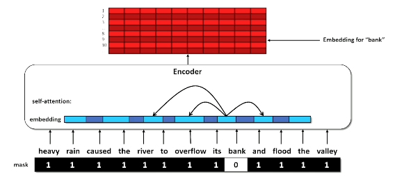
BERT uses self-attention, which means that the model can look at the words around a token (forward and backward) during inference time and factor those into the hidden state for the token.

Bert comes in many different versions:

The largest version has 345M parameters, 24 layers and 16 attention heads
Trained on a 3.4B word corpus scraped from the internet
Bert is trained by randomly masking the same word in the input and output and measuring the reconstruction loss (whether it can predict the true word)
Attention means every token encoding is a mixture of the original token encoding (via residual) plus some portion of other tokens that are being attended to

Once the model is trained:

The model can be reused for many different tasks because the corpus is very diverse
BERT pre-trained model can be downloaded and use off-the-shelf in a variety of ways
Embeddings can be used to compute word/document similarity or do retrieval
- To embed, you don’t just look up a word
- Provide a complete context span (before and after)
- Grab the hidden state for that token as the embedding
Infilling: provide a span and as mask and use BERT’s decoder prediction to guess the word
Question-Answering: question is the context and answer is masked

BERT Training Examples

Example of infilling:

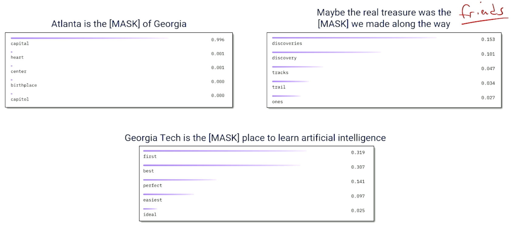
Example of question/answering:

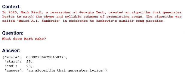
Characteristics of BERT:

One of the powers of transformers is that they can be trained on very large, diverse datasets
The contextual embedding achieved from self-attention means that the embeddings can be used for many diverse tasks and topics
Can be trained once and used for many different tasks
May still benefit from fine-tuning on specialized corpora
Fine-tuning starts from a model trained on a general, diverse corpus and continuous training on a specialized corpus to shift the parameters to achieve better loss on a specific task
BERT isn’t suited for text generation because it is Bidirectional - It can look at future tokens

GPT

Recall that BERT is bi-directional and thus is trained to look forward and backward from a masked token.
GPT tweaks to the transformer concept to make it suited for predicting the next word in a sequence
Options ($y$) are shifted to the left because we want to predict the next word
Future context is masked

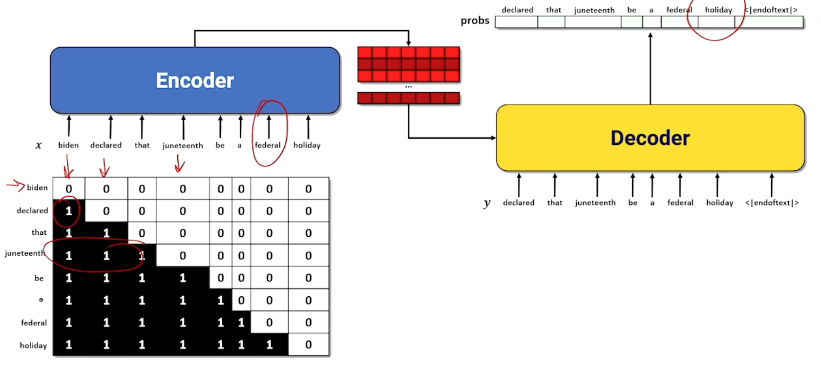
For example if we look at juneteenth, we only can look at the 3 words before that.

GPTs over time:

GPT-2:
- Released in August 2019 as a 774 million parameter model
- Was initial concern that it would be mis-used to create harm
GPT-2-Large
- Released in Nov 2019 as a 1.5b parameter model
- generally considered a good at fluent sentence completion
- Could be fine-tuned on a specialized corpus to generate texts that looked like blogs, news, articles
GPT-3
- Created June 2020 with 175b parameters
- Trained on 19B word corpus
- Not released but OpenAI provides an aPI and charges per token
- Cannot be fine-tuned because it is behind the API, but doesn’t need to be fine-tuned to do alot of things.
GPT-neo
- Created Mar 2021 with 2.7b parameters
GPT-J
- Created June 2021 with 8b parameters
GPT-NeoX
- Created April 2022 with 20b parameters
OPT
- May 2022 Facebook/Meta replicated GPT-3
- Variety of size publicly available: 125m, 350m, 1.3b, 2.7b, 6.7b, 13b, 30b, 66b, 175b
BLOOM
- Released July 2022 by 1000 AI researchers working together
- Open-access model
- 176b parameters, 59 languages, trained on 350b tokens of text from an open dataset

In summary:

Once trained, the model (GPT) can be reused for many different generation tasks
Foundation Models, large pre-trained models that are trained on a diverse enough corpus that they don’t need to be fine-tuned. Note foundation here just means “the base layer”, not like redefining things or the go to for everything.
Zero-short learning (prompting)
- GPT-3 and similar have a large context window
- Provide a prompt that includes a bunch of examples on how to perform a task and GPT-3 will “learn” the pattern and respond according to the pattern
- Embeddings are highly contextual due to self-attention so GPT picks up on the pattern
- If the model has seen something similar in the training data, then it can probable be zero-shot prompted
- Think of a prompt as an “index” into a part of the model that contains a skill

GPT Examples

Prompting / Text generation/ completion:

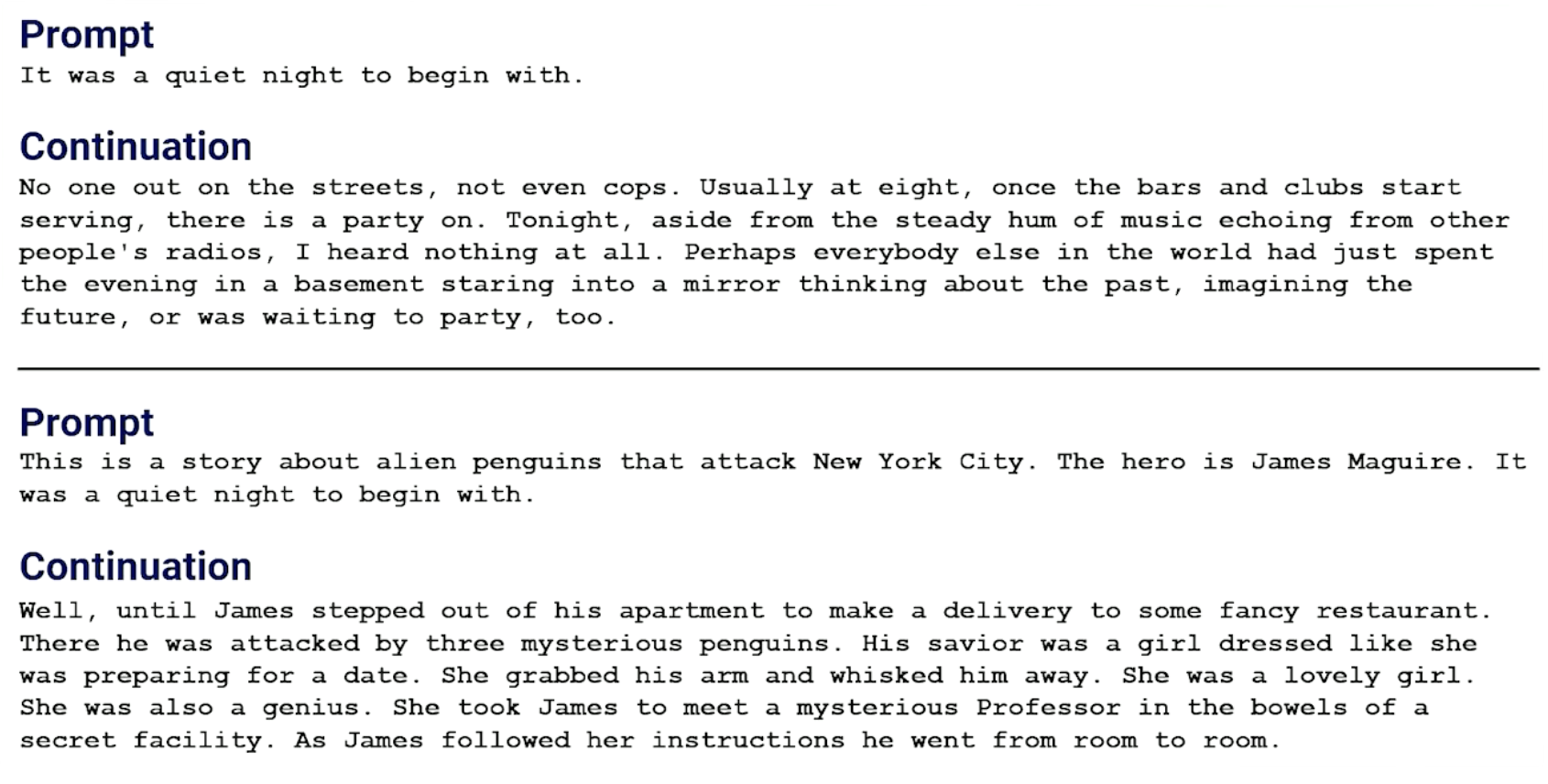
Also can be used for translation - Can see we provided examples/answers:

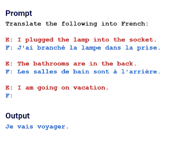
Same for open-ended question and answering:

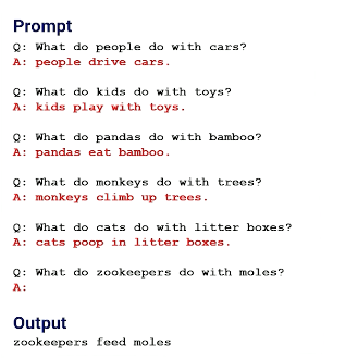
And other examples such as:

Poetry generation
Code generation
Joke generation
and others!

In summary for GPT:

Transformer designed for forward generation of continuations
Large models trained on large diverse training data are capable of generating completions about a lot of different topics
Because models now are so huge and know so many things, we find that we need to do less and less fine tuning but instead of prompt engineering - self attention makes GPT able to pick up on a pattern in the prompt and try to continue the pattern
In theory the largest versions (175b parameters) are less likely to need to be fine-tuned

Fine-Tuning and Reinforcement Learning

Pre-trained language models are trained on a large, general corpus of text and are generally capable of generating fluent text
To specialize the output, one can fine-tune the modelContinue training the pre-trained model with a small, specialized corpus
Shift the weights in the model, biasing it toward the new data

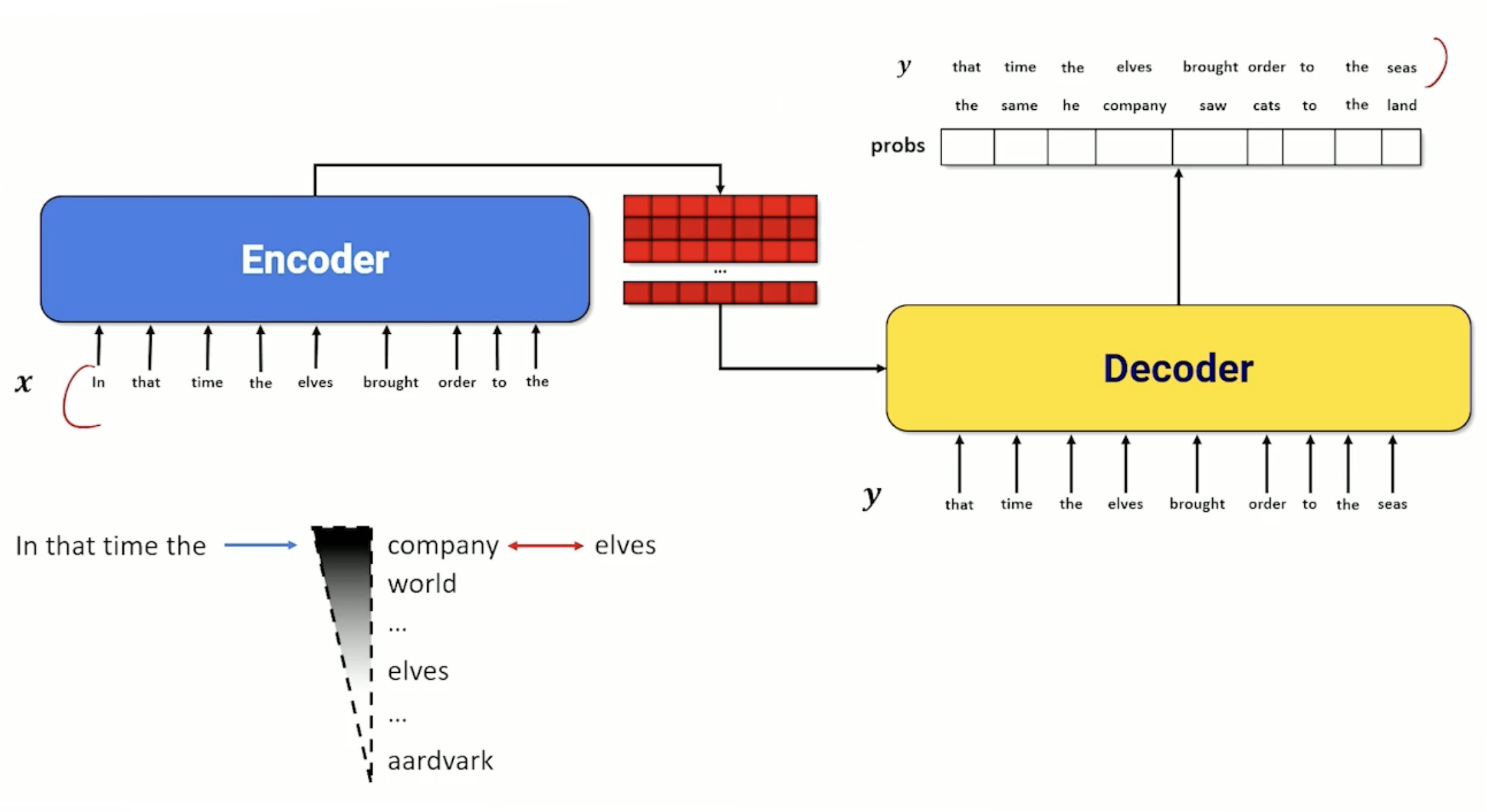
By fine tuning it, I want my language model to reflect based on my new input corpus and start changing the corpus by adjusting the probability distribution that the model outputs
E.g we want elves instead of company etc.

Now,

Fine-tuning dataset can be to small to train a fluent model on its own
The fine-tuned model will start to specialize its responses without losing the ability to respond to broader contexts
Nothing additional is needed except the pre-trained model and the new dataset.

One common question that comes up is what is the difference between prompting and tuning.

For large models (maybe >6B), then prompting may just be enough - because the models are too big and already have seen the context;
- Also usually they are too large so you need specialized hardware.
If you need specialized tasks/info and prompting will not be able to accomplish what you need, so you have to resort to tuning and providing your own dataset.

Instruction Tuning

Special version of fine tuning, let’s look at an example:

Prompt: “Write an essay about Alexander Hamilton”
Response: “Include at least two references and full bibliographic information”
- This seems unexpected, why?
- Turns out it is treating it like a prefix and treating it like a classroom assignment and provide the rest of the classroom assignment
The problem is that the most probable continuation, based on all the times it has seen the prompt is not the same as treating the prompt as an instruction

Here how is to handle instruction tunning:

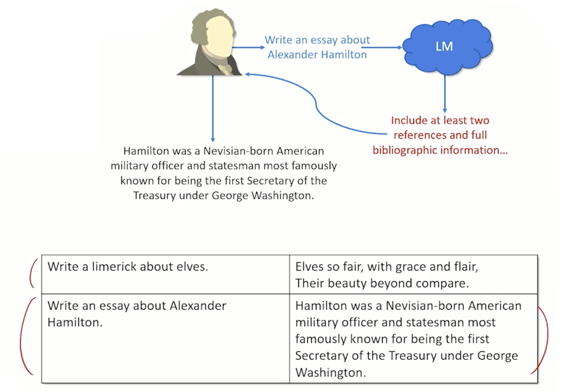
Human prompts the model
Model returns response
Humans correct the output
Collect up corrections into a new dataset
Fine tune on corrections

Reinforcement Learning

What if we have human feedback of the form / ?
Instruct tuning doesn’t work

There is another thing we can do beyond instruction tunning - reinforcement with human feedback.

Reinforcement learning solves a Markov Decision Process (MDP) by performing trial-and-error learning with sparse feedback
- Don’t need to know much about MDP
Agent must figure out which action will get it the maximum amount of future reward
A reward function sometimes give a positive or negative value to a state or action, but most of the time does not provide any feedback
Explore different actions until something provides reward
Try to learn what you did right (or wrong) and do more (or less) of that reward

Reinforcement Learning for Text

Pretend each token generated by a language model is an action
Agent generates some tokens for a while and then receives rewards
Need to somehow convert rewards to loss (reward = 0 is bad, loss 0 is good)

Example one:

Prompt: “What is Mark Riedl famous for?”
Output: “Mark Riedl has research automated story generation, graphics, and reinforcement learning”
Feedback:
The problem is the statement isn’t exactly entirely wrong, only the “Graphics” portion is wrong.
So, how did the system/model know which word(s) was/where wrong?

Problem one: Which word (Action) should get the negative reward?

If I punish every token in the sequence, it will not generate the things that are correct
Solution - Explore different variations
- “Mark Riedl has researched automated story generation, safety, and reinforcement learning”
- “Mark Riedl has abandoned automation story generation, graphics, and reinforcement learning”
- Which leads us to the next problem

Problem two: No human feedback for variations, The solution:

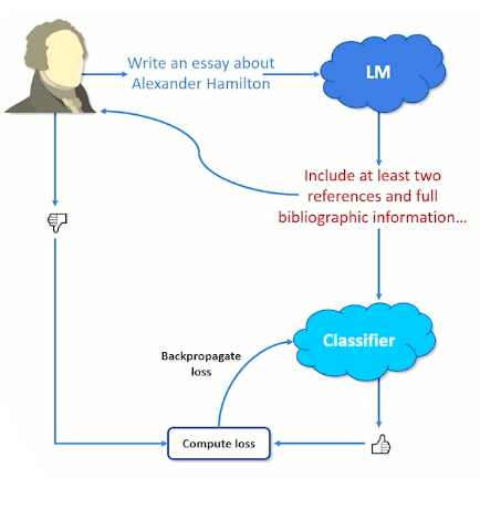
Train a classifier on human feedback
User prompts model
Receives response
Provide / feedback
Classifier attempts to guess / and loss is backpropagated

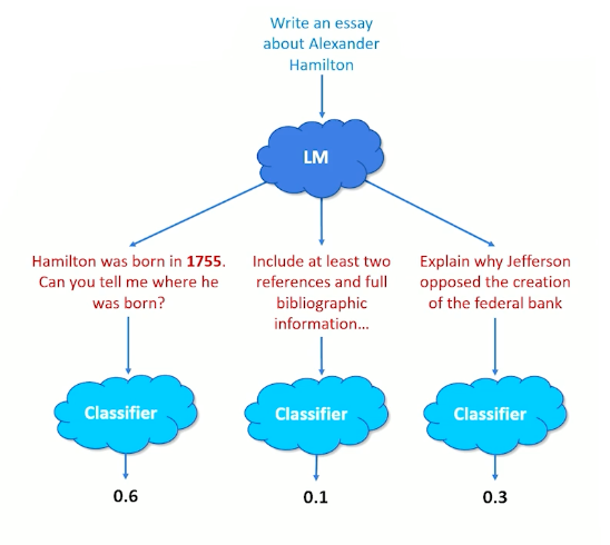
Feed text into LM
Generate multiple response
Score each response with the classifier
Use score (probability output) as replacement for human feedback

In summary:

Sometimes a prompt is an instruction it is the first part of a pattern to continue, and sometimes a bit of both
A LM (language model) doesn’t understand the intention of the input, which means it can respond inappropriately
Tuning the model shifts the parameters ot prefer one way of responding (token choice) over another
Generally, people report that “instruction-tuned” models feel more like they are listening
Can also reduce toxicity, reduce prejudicial bias, and other “unsafe” outputs (e.g talk about suicide)
Downside: Need to collect a lot of human feedback, regardless of whether instruction-tuning or using reinforcement learning

Transformer Code

For the next 3 sections in Module6, just refer to the python notebook over at Transformer Walkthrough Code

Code Analysis Introduction

Just note the different hyperparameters:

  


d_embed = 512       # embedding size for the attention modules
num_heads = 8       # Number of attention heads
num_batches = 1     # number of batches (1 makes it easier to see what is going on)
vocab = 50000       # vocab size
max_len = 5000      # Max length of TODO what exactly?
n_layers = 1        # number of attention layers (not used but would be an expected hyper-parameter)
d_ff = 2048         # hidden state size in the feed forward layers
epsilon = 1e-6      # epsilon to use when we need a small non-zero number

Make dummy data
Encoder

Code Analysis: Self-Attention Module

Self attention module (Section 1.2)
Final Encoder Layer Normalization (Section 1.3)

Code Analysis: Decoder

Decoder (Section 2)
Generate Probability Distribution (Section 3)

Module 7: Information Retrieval (Meta AI)

Classical Information Retrieval

Information retrieval means searching for relevant information which satisfies information need
Usually from a large collection of text documents
Most notably the web, but also emails, personal/work documents, legal. ….
Arguably the defining task of the information age.

We will go through the basic task definition and also a few retrieval paradigms:

boolean retrieval
Ranked retrieval
Vector-space models
Probalistic IR

As well as metrics and evaluation

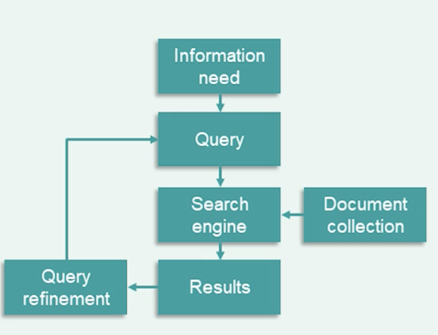
For the task of information retrieval:

Assume fixed set of documents for now
Example user information need:
- “Find out when my NAACL paper is due”
- Example query: “naccl dates”

At the heart of information retrieval system, a document d, given query q is relevant, if it satisfies the user information need and not relevant otherwise.

Note, relevance is defined with respect to the original information need, and only indirectly relates to the query
- e.g document containing the terms “naacl”, “dates” could be irrelevant, if it doesn’t contain the actual paper deadline
- Relevance can be ambiguous
  - Which date am I looking for?
  - Which year?

Before diving deeper, we need to understand precision and recall:

Given set of results document, $R = {d_1,…,d_n}$
Precision : Of all documents in $R$, what fraction are relevant?
Recall: of all documents which are relevant in the collection, what fraction appears in $R$.

The simplest way of implementing text retrieval is by matching terms of words in the query to terms in the document, known as term-matching methods. For example:

How to search for terms (“naccl”,”dates”) in documents?
Searching through all documents is slow
Return documents with naacl AND dates?
- How about more complicated queries like OR, or naccl and NOT 2021 etc.
Efficient implementation of such systems need to pre-compute and store term inclusion in documents so queries can be executed faster.

Term-document incidence matrix

The data structure which stores the inclusion of each term for each document is called the term-document incidence matrix.

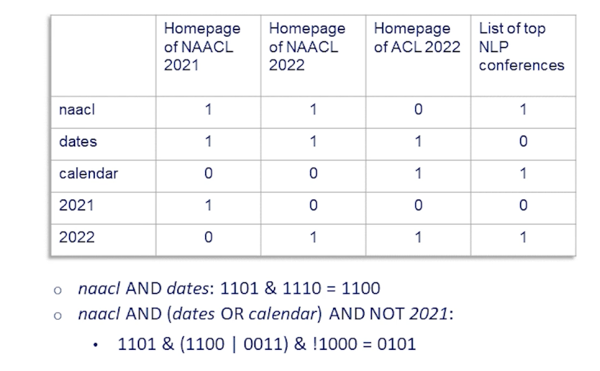
Each column in this matrix is a document, and the number of columns will be the number of documents in the collection.

Each row is a term or a word, any term which appears anywhere in the collection will have a row in this table, and the number of rows is equal to the number of unique terms that appear in the collection.

The entires in this matrix are binary, if a term appears in that particular document, the entry is one, otherwise it is zero.

So, given such a term-document incidence matrix, we can quickly see how to calculate the set of documents, which are both naacl and dates.

we simply take the binary row vectors corresponding to naacl and dates and perform a bitwise and operation.
The resulting binary vector indicates the relevant documents. In this case only the first two contain both naacl and dates.
- Extends to other type of queries as well.

This idea is pretty simple, but:

Problem: term-document matrix can be too large even for moderate size collection
Case study: As of 7 march 2022, there are over 6million English Wikipedia containing over 4 billion words
If we assume 1 million unique terms, that’s over 6.5 trillion bits to store
- And if we talk about the web, it is even larger.

So what can we do to reduce this search space? one stright forward way is to use term normalization

Lower case, drop punctuation
- e.g Ke$ha $\rightarrow$ kesha
Stemmization, lemmatization
- am, are, is $\rightarrow$ be
- organizes, organizing $\rightarrow$ organize
Remove stop words
- The, a, of , …
Highly language dependent
Precision-recall tradeoff
but…. Index still too large.

One critical observation we have to make to address this problem the term document index matrix is sparse.

For example in wikipedia if each article only has 630 words over 1 million vocabulary, over 93% bits is not required.

We can overcome this with the inverted index, it consist of an index of terms, for each term, store indices of documents which it appears in (sorted)

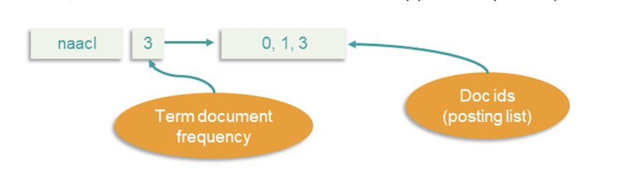
This is also known as the posting list
It also stores the term document frequency

Supporting boolean queries with this matrix can be done as follows:

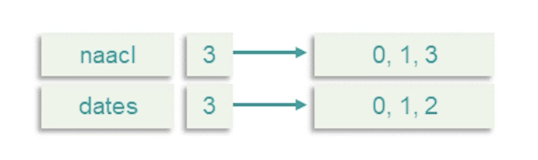
Each doc is a bag of words
Process AND queries by merging lists
- Linear of $L_1 + L_2$ (Why we sort)
- See that we still retrieve the first two documents (0,1)
Can also do OR, NOT, recursive
Optimize by doing rarer terms first (Why we store document frequency)
Boolean search with inverted index was the dominant IR tool for decades
- still used for email, document search etc.

Phrase Queries One question/problem that comes up is what about phrased queries (multiple words)?

How to handle “red hot chilli peppers”?
Can index all n-grams as terms
- But this is way too large
Instead, we can index bi-grams, chain them together:
- “red hot”, “hot chilli”, “chilli peppers”
- Can have false positives
- But even so, the number of indexes are still too many
Solution?
- Use positional index.

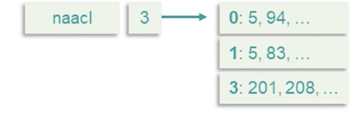
Store the index of each position the term appears in the document
Can use a two-stage merge algorithm to support phrase queries
Can also support proximity searches

The clear drawback of positional indices is their complexity.

There are 2-4x larger than regular term index (roughly 50% of original text size)
- Frequent terms are especially expensive
- Can use compression to reduce size
Can be combined with bi-gram index
- Index popular bi grams (e.g Michael Jackson) as terms.

Ranked Retrieval

In practice, we care about the order of documents.

Boolean search often results in a feast (too many results) or famine (too few results)
Good for experts
- Know how to formulate query to get manageable results
- Get exactly what you search for
Good for machines
- sift through 1000 of results
Not great for people

Introducing Rank retrieval:

Return a ranked list of results, sorted according to relevance
More user friendly
- Manageable top-k list of Results
- Uses free text query vs Boolean operators

Term-Frequency Inverse-Document Frequency (TF-IDF)

\[TF-IDF score = \sum_{t\in q \cap d} 1 + log\ {tf}_{t,d} \ times log_{10} \frac{N}{df_t}\]

Best invented weighting heuristic in IR
Many variants
- with/without logs
- Can also weigh query terms

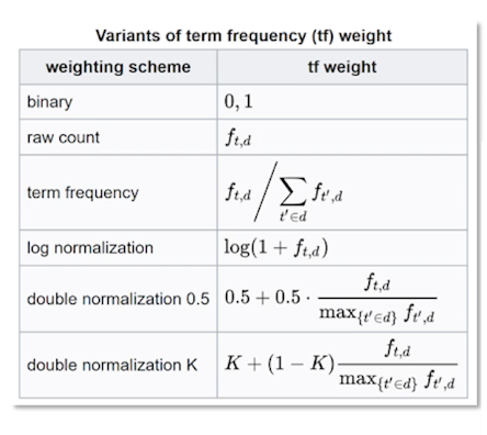
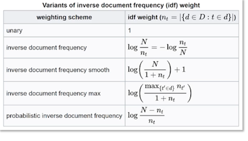
Choosing which one to use is a matter of experimentation.

Revisiting our term document incidence matrix:

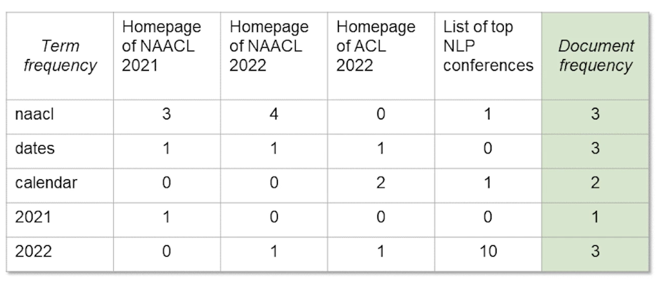
To calculate TF-IDF, for each cell, you see we calculated the log term frequency multiplied by the log inverse document frequency, then given a query, its just a matter of summing up the TF-IDF values for each term in the query.

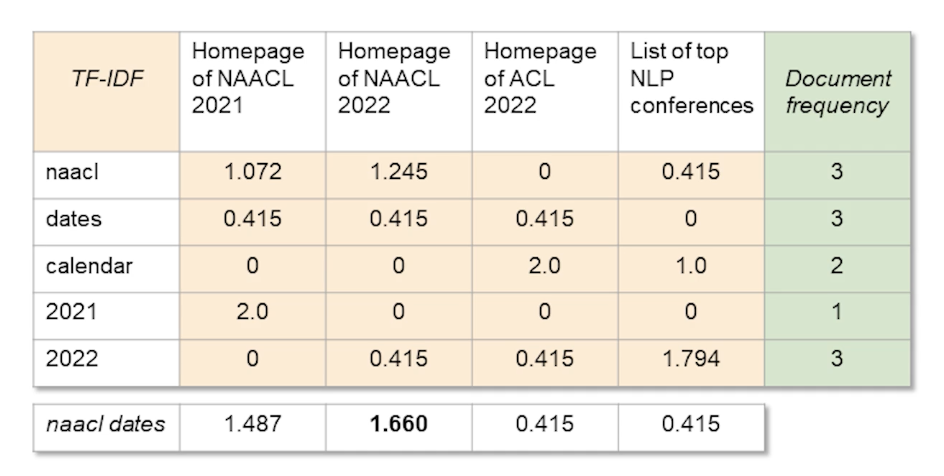
We still see the first and second document being ranked as top 2, which is expected.

Probalistic Information Retrieval

In probabilistic information retrieval,

Relevance is ambiguous and hard to defined
A statistical approach seems apt
Rank documents by probablity of relevance
- $P(R = 1 \lvert d,q)$
How to model $P$?

Lets look at the simplest approach: Binary independence model.

Here we just consider the query and documents as represented by a bag of words. The order of terms does not matter and we can just represent the document type query by the term incidence vector. This is just a binary vector of zeroes and ones, the size of which is the vocabulary size. Each entry is one if the term appears in the document and 0 otherwise.

Moreover, we assume that they appear independently of each other given the query and relevance label, and this is the critical assumption behind this binary model. With this assumption and this formation, let’s see what the relevance probabilities end up looking like:

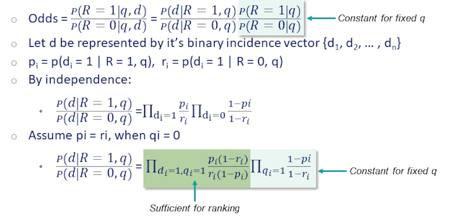
We will look at the odds of a document being relevant. We will look at the odds of a document being relevant. In other words, how much more likely is it that this document is relevant than it is not relevant. We will use this as our ranking score function.

Ranking by the odds is clearly equivalent to ranking by probability of relevance, but makes the math a little cleaner. If we break down the probabilities by the chain rule, we get two terms, The second one is the odds of relevance condition on the query only. Since this is fixed for a given query, it has no effect on the ranking, so we can safely ignore it for our purposes.

The first term, is the probability of generating a document conditioned on the query and condition on the relevance label. For the binary independence model, since we assume term incidents to be independent, we can factor this probability for each term. We introduce a little bit of notation here to make the equations easier to follow.

Let $P_i$ be the probability of term $i$ appearing in the document given the document is relevant. And similarly, $r_i$ is the probability of the term appearing given that the document is not relevant. These corresponds to the quantities in the numerator and denominator of our ranking score respectively.

Using the independence assumption now we can break down the fraction into product over all term indices and also group the product for term indices which are one which appear in the document and term indices which don’t appear.

Now, lets consider the case that $q_i = 0$, in other words, a term which does not appear in the query. To further simplify things, we assume these terms don’t give us any information, they appear with equal probability whether the document is relevant or not. With this assumption, we can regroup the terms to come up with this final equation here, which is highlighted. This is the product overcoming terms which appear in both $d$ and $q$ multiplied by another product which is over the query terms only. We notice that the second term is constant for a fixed query, therefore it has no effect on ranking, and that leaves us with just the first product which conveniently only consider terms that are common to documents and query.

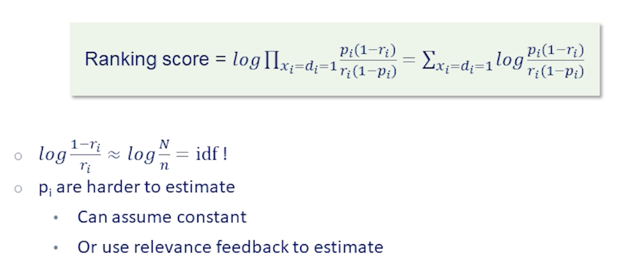
So lets take a closer look at this ranking term, Taking logarithms, we end up with a sum of scores and two terms that appear in the score. One is $\frac{1-r_i}{r_i}$, recall that this represent terms probabilities in the not relevant case. In this case, the probabilities should be approximated as the unconditional probability of this term, since the vast majority of documents will not be relevant. Since most terms appear only in a small fraction of documents, $r_i$ is smaller, this fraction should be very close to inverse document frequency. So this provides a very nice justification for the IDF term in TF-IDF.

The second term, the term involves $p_i$’s is tricker to estimate. So recall that $p_i$ is the probability of a term $i$ appearing indicates the raw document is relevant. Intuitively, this should be a non-trivial probability as we’re expecting a query term that appear in relevant documents with significant probability. If we have a training set with relevance labels, we can try to estimate this probability. Otherwise we can just say $\frac{p_i}{1-p_i}$ to be a constant and hope for the best.

Probalistic Information Retrieval (BM25)

The BIM (binary independence model) is a very simple ranking model, and makes a bunch of assumptions, some of which are justified in in practice and some of which might not be.

For instance, the independence of terms in documents is a very strong assumption which help keep the math simple, but almost surely not accurate in practice.

Another assumption is that terms that do not appear in the query do not appear the ranking. It i is easy to think of counter examples, for example, synonyms or translate it to the query terms but are not exactly the same, should surely affect the document ranking.

The boolean bag of words representation for queries and documents is yet another simplification, which is not neccesarily accurate. There are cases where word or order / freuqencies matters as in often used example, man bites dog versus dog bites man. We’ve talked about booelean relevance, and there are more fine main notions of relevance which can capture this document is more relevant than that document.

Finally, the assumption that the relevance of each document is indpendent, this one intuitively make sense but when you consider the value of the set of results that we return rather than each document in isolation, then it’s actually better to consider overlap and diversity between documents. For instance, if there are duplicates in our collection of documents, won’t add any value to return a bunch of those in the result set.

So, clearly the BIM model can be improved in various way and we will look at how to remove at least some of these assumptions.

BM25

One such model is what is called the BM25 Model, which stands for best match 25 since the authors tried a lot of variants and arrived at the 25th try.

Generative document model similar to BIM in words that drawn IID from multinomial distribution.
In contrast to BIM, term frequency is not Boolean by this model as mixture of two poisson distribution depending on whether the term is elite or not.
- Elite word here means terms which are specific to the central topic that the document is about versus other terms which the document just happen to mention. Each document is assumed to be composed of these two groups of terms.
The log odds ratio is approximated by $\frac{tf}{k+tf}$ where k is some constant.
- This is function is increasing return frequency and it saturates at one, and k is a parameter which controls slope of this function and can be set empirically.
- The rest of derivation is similar to the beam model.

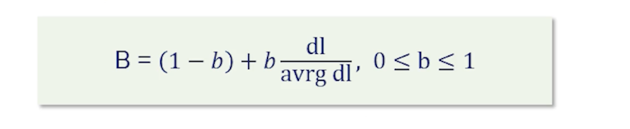
So far we have not really considered the effect of document length.

Longer document are more likely to have higher term frequency, it might make sense to normalize term frequency with document length.
- however hte effect might be more complex, for example longer documents may have larger score, in which case they might be more likely to be relevant.
- But they could also just be more spammy nad repetitive in which case they are less likely to be relevant.
The solution here is to normalize to some extent but set the normalization parameter empirically. In this case, we set a parameter b between zero and one, where zero means normalization and one means normalization proportionally to document plans.

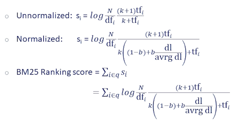
Putting that together, at the top we see the expression for the score rebuild without document length representation. Consists of the inverse document frequency term, which follows from the independence of terms as we saw in the BIM derivation.

We also see the term frequency appealing, which we just talked about, which comes from the poisson mixture approximation. As you can see, after all that meandering, it ends up looking very similar to TF-IDF, just some more smoothing provided by this parameter k. Now on top of that, we add the document length normalization, which normalizes both term frequency terms in that direction, and that gives us the full BM25 ranking score.

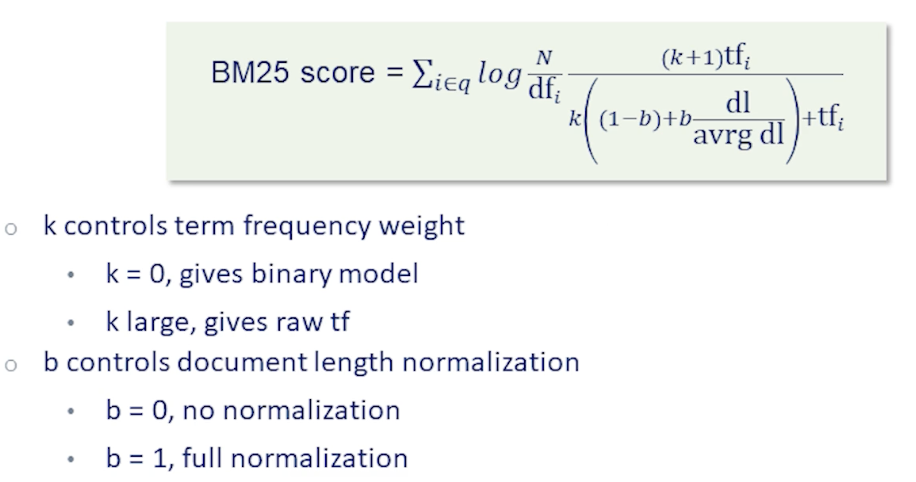
This BM25 model has a total of just two free parameters which can be determined from data.

k control term frequency weight
- k = 0, gives binary model
- k large, gives raw tf
b controls document length normalization,
- b = 0, no normalization,
- b = 1, full normalization

Metrics and Evaluation

To measure performance, we need datasets in information retrieval that takes the form of a search relevance dataset. Such a benchmark dataset consists of the following:

A document collection ( e.g wikipedia articles, news articles, etc…)
A set of queries
- Ideally samples from real user queries
Relevance labels for each (q,d) pair
- Could be binary or more nuanced

Given such a dataset with adequate size, we can build, run, and evaluate information retrieval models. However,

Infeasible to label all (q,d) pairs, even with crowd sourcing
Instead, fetch likely candidates (by using a simple model like TF-IDF), only label those
- needs a working IR system (model bias), which leads to bias to generate these initial candidates. Clearly all (q,d) pairs we label has to come from retrieval results of this basic model. And conversely if this model is unable to to retrieve the correct documents for subqueries, those will not appear in our datasets.
- There will be false negatives, and there will be bias.
  - Unfortunately there is no easy solution other than making sure you label enough candidates from this baseline model.

Example of relevance datasets:

Some of the most popular and earliest examples of relevant data sets were produced for the TREC Text REtrieval Conference. This conference rose in popularity with that advance and success of web search engines as multiple tracks for web search, deep learning models, question-answering legal medical domains etc.

One of the largest pops in information retrieval benchmark is the MSMARCO dataset from Microsoft. This dataset consists of almost million queries from real search logs of tubing search engine coupled with 8.8 million excerpts or passages from web pages retrieved by being for these queries. The dataset comes with multiple relevance labels for each query and also includes human-written free-text answers to a subset of queries which are posed as questions.

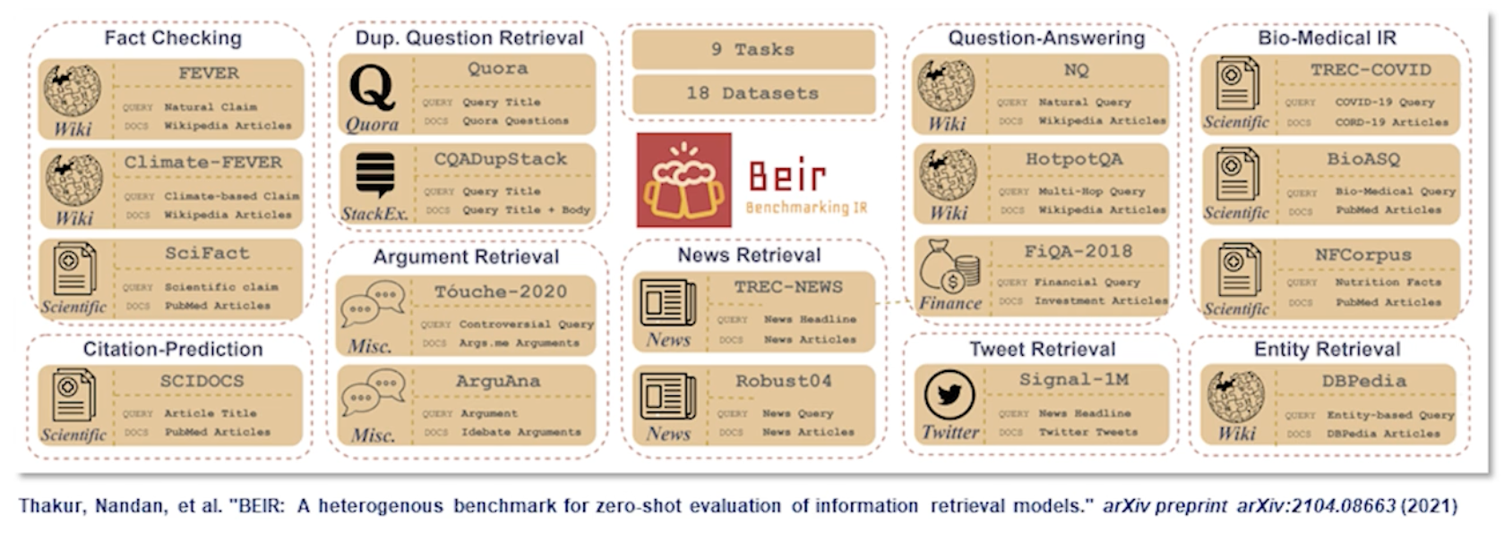
A more recent benchmark or rather a collection of benchmarks for retrieval is BEIR. BEIR collects together IR data sets from diverse set of domains such as web search tweets news or scientific articles. The original motivation for the benchmark was to evaluate generalizability of retrieval systems to new and unseen domains. This continues to be an active research area.

Metrics

A good retrieval system should put relevant documents above non-relevant ones. There are various metrics to quantify this idea. To recap Binary legitmate metrics precision:

Binary IR metrics
- precision, recall
Ranking metrics
- Precision at K - the ratio of correctly identified relevant items within the total recommended items inside the K-long list
- MAP (mean average precision)
- MRR (Mean Reciprocal Rank)
- NDCG (Normalized discounted cumulative gain)

Precision at K PR@K and MAP

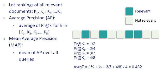
If we have an ordered set of documents we can calculate precision for the top k documents returned for any k. We refer to this metric as precision at k.

Precision at k is obviously a function of which k we pick. Should we look at just the top from k=1 or should we use k=10? A model might be better for one but not the other. Sometimes we know what k makes most sense for our application for instance we might be presenting 10 results in the first page of results in which case k=10 equals might be a good choice. However sometimes it is desirable to have a single metric to pick the best model overall.

Mean average precision or MAP is one such metric. MAP is the average of precision values at values of k which correspond to the ranking of the relevant documents. In this example there are four relevant documents:

Their ranks are 2, 4, 7, 8
Calculating precision values at those rank which is 1/2,2/4,3/7,4/8
Which gives average precision of 0.482
MAP (Mean average precision) is the mean of average precisions for over all queries in our evaluation dataset.

If there are no relevant documents in the results the mean average precision is clearly zero. Also note that the contributions corresponding to each relevant document in the results is weighted equally. So this assumes the user is interested in all the relevant documents which might or might not be the case.

Another drawback of MAP is that it works best when there are many relevant labels in our dataset for each query.

MRR - Mean Reciprocal Rank

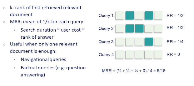
Mean reciprocal rank, or MRR, only considers the first relevant result. It’s defined as one over the rank of the first relevant result averaged over all queries. This is motivated by applications where a single relevant result is usually able to satisfy the users information need. For instance for a web search we’re usually not interested in reading all the web pages which might be relevant once we find the information we’re looking for. Also if we assume the user is scanning results from top to bottom the rank of the first relevant result should be correlated to the time and effort spend by the user to find what he or she is looking for. This justifies the use of reciprocal rank metric as a proxy for user effort.

NDCG - Normalized discounted cumulative gain

Normalized discounted cumulative gain or NDCG is another often used metric for retrieval. It is the only one we’ll cover which takes into account non-binary relevance ratings ${0,1,2,…}$.

Which means it can discriminate between highly relevant documents and just moderately relevant ones.
Another property of this metric is that it assumes lower-ranked documents are less useful to the user similar in spirit to MRR.
Ratings in ranked order for top n docs: $r_1,…,r_n$
cumulative gain $(CG) = r_1 + … + r_n$
- If this is binary, is equivalent to using precision at n.
However, since we higher ranked documents to be more important, we can discount them by rank and then sum them:
Discounted CG = $r_1 + r+2/log 2 + …, r_n/log_n$ $DCG = r_1 + \sum_{i=2}^n \frac{r_i}{log i}$

NDCG:

Normalize DCG at rank n by the ground truth, maximal, DCG value at rank N
Useful for queries with a varying number of relevant results
- Notice that the discounting here is logarithmic, whereas in MRR it was linear.
- So NDCGS discounting is more mild than MRR

The last step is to normalize the discounted cumulative gain by the maximum value at each rank. How do you find this maximum value? We take the best possible ranking that is rank all documents in order of their relevance labels and calculate DCG on this ground through ranking. Normalizing in this way is useful to have consistency with queries having different numbers of relevance labels and relevant results. It also ensures the value is always between zero and one.

An Example:

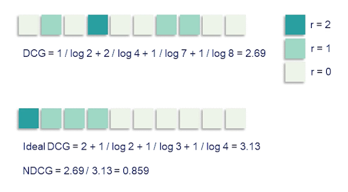
We have three levels of relevance here with r equals 2 being most relevant shown by the dark green squares r=1 is medium relevance shown in a lighter green and r=0, not relevant, are the light squares.

We have three medium-relevance documents and one high-relevance one in this example. If we just sum up the ratings that would give us cumulative gain and that would be equal to five in this example.

To get discounted cumulative gain we divide by the log ranks for instance the first medium relevance document is at Rank 2 so we divide it’s rating by log of 2 and so on giving us a DCG value of 2.69. In the below figure we show the ideal ranking. So here we ordered documents by the labeled relevance ratings. We can recalculate DCG for this ranking which of course results in the higher value of 3.13. Normalizing 2.69 by 3.13 gives us the NDCG metric value which 0.859.

So relevance benchmark datasets are a good way to measure progress especially in IR research but at the end of the day what we care about is real user value from an online system such as a search engine. When we have a working system with users there are more direct ways to measure improvements by leveraging feedback from the user such as click data which are cheap and plentiful. We won’t talk about this topic in any detail but I wanted to give one example how one could make use of this to compare two retrieval models in an online setting.

Say we have two competing ranking algorithms and want to decide which is best. What we can do is combine results from both systems and present the interleaved results to the user in random order. Then we aggregate clicks while tracking which result comes from which model. At the end of the day the algorithm with the most clicks wins. This is a very simple instance of what we call A/B testing which is the main method by which commercial IR deployments are tested and evaluated and improved.

We are at the end of our lecture on classical information retrieval methods.

We’ve talked a lot about term-matching methods which are simple and powerful at the same time. However, these methods only rely on the surface form of words and have no deeper understanding of semantics These methods don’t work well with natural language and instead prefer a list of keywords. With the increasing volume of data that we have we can start building better models which understand things like context and synonyms and can work well with natural questions directly return answers to user queries using tools from machine learning and deep learning. This course is about natural language processing and in the next lecture hopefully we’ll talk about how machine learning and natural language process methods are used in retrieval systems

Neural Information Retrieval

Information retrieval is the task of searching for and retrieving relevant information which satisfies the user’s information needs. Information retrieval models are everywhere and the web as we know it would not function without them since there’s so much information out there there is simply no way of getting value out of that without retrieval.

Previously we discussed the foundations of information retrieval and covered term-matching heuristics like TFIDF which are very robust and effective and have been the dominant tool in IR until recent years. Now we will go back to the origin trade-off of this lecture series and see how tools from machine learning and NLP can help improve retrieval models.

First we will look at Machine Learning for IR (aka Learning to rank)
Retrieve and rank pipeline
Embedding based IR
Neural retrieval (Neural Network Methods)

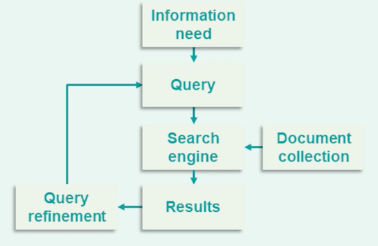
Here’s the outline of a typical IR system. Classical text search engines have been heavily dependent on text matching heuristics such as TF-IDF which decide documents relevance based on whether the document contains terms exactly match the terms which appear in the user’s query.

However we all know modern search engines are a lot more complicated than this. First of all we usually have access to a lot more information than just takes the query and documents. For example we might know information about the domain from which to a page counts from, the freshness of the context. We can extract PageRank and information from hyperlinks pictures and potentially hundreds of more features.

There is no way for a term matching system to make use of this information. Moreover we have a lot of data in the form of user click logs and large labeled retrieval datasets which we can and should use to make our models a lot more precise. TF-IDF variants are robust but rigid and cannot really make use of any of this information. Instead we can use powerful machine-learning algorithms, gradient boosted decision trees, neural networks to learn from this vast amount of information and build information retrieval systems which better understand and fulfill the user’s information needs.

To see how information retrieval can be cast as a machine learning problem consider the ranking model

For each $(q,d)$ pair consider a function:
- $f(q,d)\rightarrow s$, where $s$ is a relevance label
$s \in {0,1}$: binary relevance (binary classification)
$s \in {0,1,…,k}$: multi level relevance (multi-class classification)
$s \in \mathbb{R}$: binary relevance (regression)

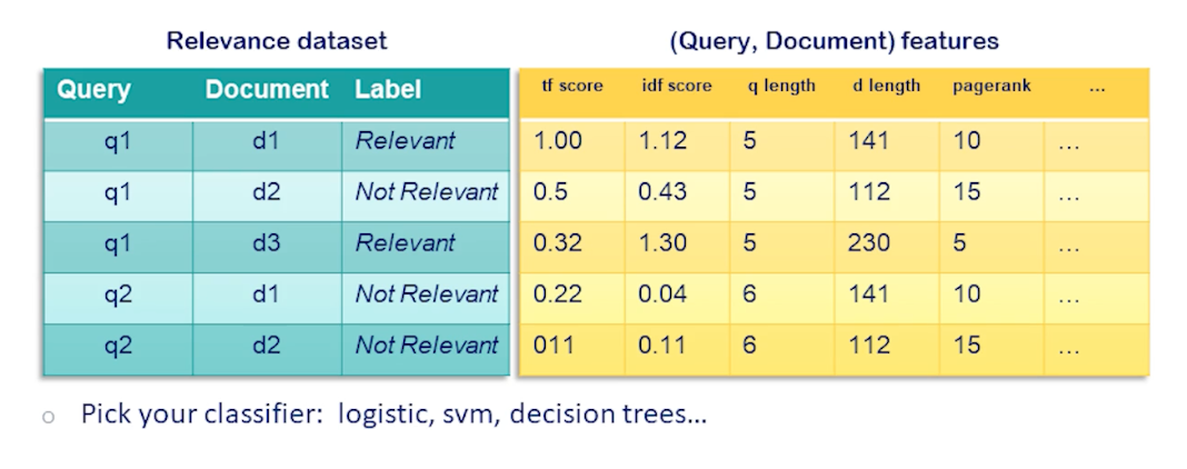
Here is how we would train such a model. Suppose we have a standard search relevance dataset comprised of (q,d) query document pairs and the relevance label for each row. We combine this with a table of features that we extract from each query document pair. We can include our regular text matching scores here like tf, term frequency, and IDF, documents frequency, at other query and document level features such as query and document lengths, PageRank, freshness of the document etc. We could even include user features or location features for personalization. At this point we have a complete dataset for training a machine learning model and we can pick our favorite algorithm to do that be it logistic regression SVMs decision trees or anything else.

Reranking pipeline

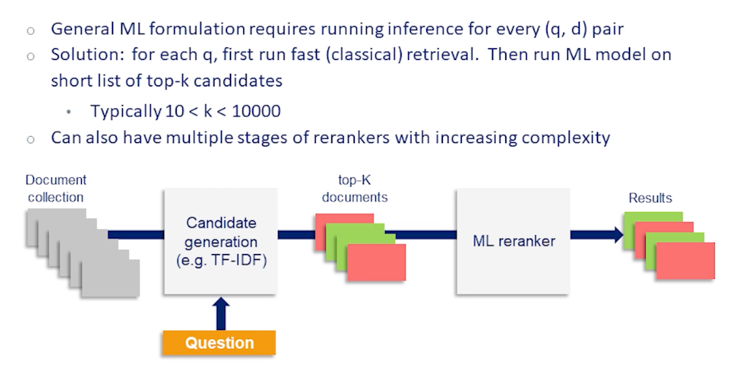
Training your model in this way is conceptually simple.

However it would not be possible to name this such model since each query we would need to run the model on every document in the collection to calculate the ranking. Remember that the classical information retrieval methods that we covered in the last lecture I designed for fast retrieval from start making use of very simple heuristics and efficient data structures such as inverted indices to return results quickly even for huge document correlations. By using machine learning algorithms obviously introduces a lot of complexity and how to incorporate that without ballooning the computational cost needed samples.

The simplest way of making use of machine learning models is to incorporate them in a reranking setup. In any ranking pipeline we rank documents in two steps. In the first step we reduce the large collection of documents into a shortlist of potential relevant candidates. For this step we need to use a fast retrieval heuristics such as TF-IDF. But in the second step since the number of documents now is more manageable anywhere between K=10 to a few thousands of documents we can use our trained machine learning models to score each candidate documentaries respect to the query and to re-rank them. If the recall of our first-stage system is adequate then we get both the advantages of using a powerful model and manageable latency we get from the past first stage retrieval system. We can also add even more steps of reranking where at each stage we shrink to pull off candidate documents but the model we use increases in complexity and cost. Thus the reranking pipeline is neat and often used way to trade off computational cost and accuracy in the retrieval system.

From Classification to Ranking

In previous sections we saw that information retrieval can be cast as as a classification problem. However this is not the most natural formulation

classification only defined an absolute notion of relevance
Ranking requires us to consider not only whether a document is relevant
- but also if it is more or less relevant than competing documents
In practice classification is
- good for discriminating random irrelevant documents
- but not for superficially relevant onw
To overcome these issues native ranking methods have been introduced.
- An example is using pair-ranking objectives instead of a point objective ranking classification
- Another technique is using hard negative examples
  - which are documents which looks superficially relevant but don’t really answer the query and show as false positives
  - Using these difficult examples and training can help the model learn a more fine notion of ranking

So to make things concrete let’s go through the components of as simple logistic regression classification model and compare it to an equivalent pair-ranking set up.

In classification the quantity of interest that we’re predicting is probable to of relevance given a query document pair the scoring function takes in a single query document pair and output a single score $s_i$ which is essentially a point estimate for each document $d_i$. Then the model is say the probability is equal to the sigmoid or the score function.

So to train this model we have a list of documents with binary relevance labels. The labels evaluate each document independently. The loss is cross entropy loss which is just the log probability of the correct labels under our model which is log of sigmoid of s in this case if the label y is 1 or log of 1 minus sigmoid of s, y is 0. After simplifying that a little bit that comes $1-y_i$ times $S_i$ minus log of sigmoid $s_i$. Now if you look at the gradients of the loss with respect to the model parameters w we simply get the derivative of the score function with respect to w multiplied by the error which is the difference between our predictions sigmoid $s_i$ minus the label $y_i$. This Lambda or the error determines the step we take training the model with gradient descent.

Now in the pair-ranking set up instead of modelling the relevance probability of a single document in isolation we model given two documents, the first document is more relevant than the other. You can still use a point-wise scoring function as in the classification case but the model now takes two sides scores in the sigmoid. The problem desired the highest score difference between the two documents. The labels are also different. Instead of labeling each document in isolation we ask greatest peak the more relevant one out of two documents. Having raters rate this way actually can improve data quality and interleaving agreement since it is usually easier to compare two documents than to assign an absolute rating to one on it’s own. So the label $y_{i,j}=1$ if $d_i$ is more relevant than $d_j$ and zero otherwise. Most calculation is identical only replace the $s_i$ in the sigmoid. Now the margin or difference $s_i-s_j$ and similarly for the lowest grade. In the end if you look at the expression for the gradient you get the expression for the step size Lambda but this time it’s a function of the pair of documents i and j and represents the error of the pair prediction rather than the points prediction.

Ranknet

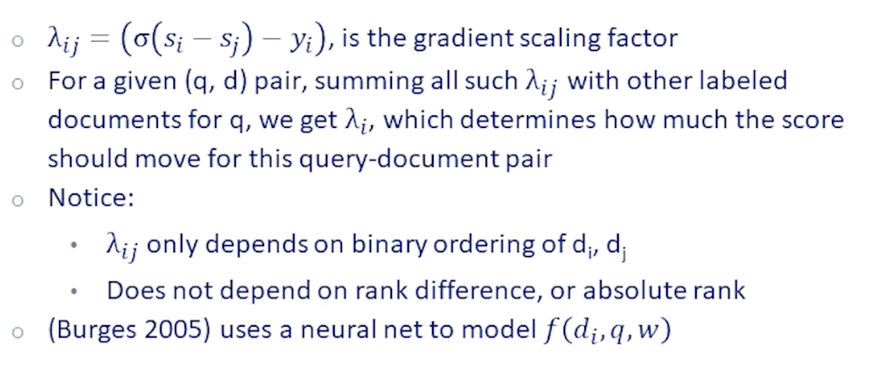
An early example of learning to rank algorithm is RankNet which was based on pair-ranking ideas. To calculate score gradient for a given query doctrine pair we consider the sum of all such $\lambda_{ij}$s for all labeled documents paired with q. Note that $\lambda_{ij}$ only depends on the binary ordering of $d_i$ and $d_j$. And in particular it does not depend on their rank difference or absolute ranking. So whether d_i is ranked first or tenth or whether $d_j$ is ranked 500th will not make a difference in the score. Also as a side note this early paper used a neural network to model the scoring function.

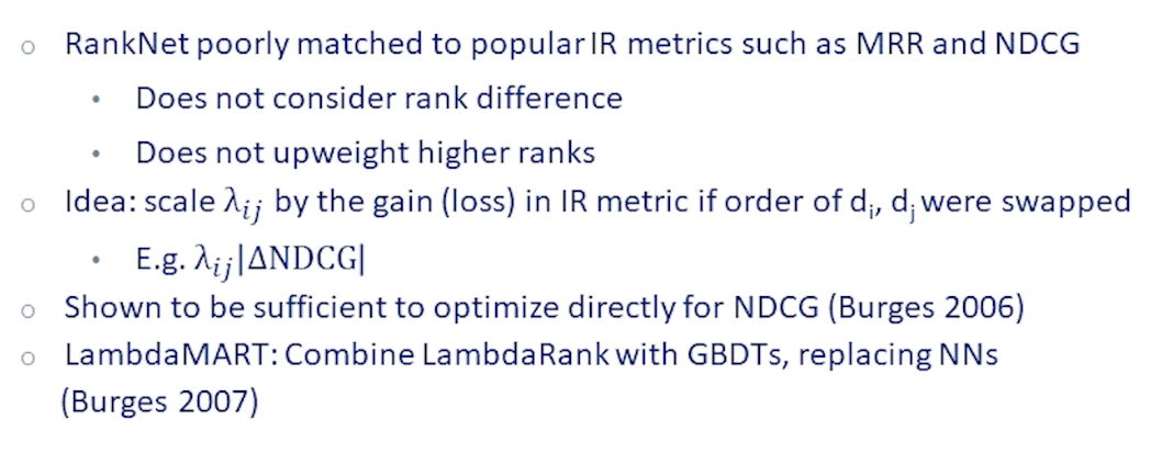
The more famous example is LambdaRank and it’s variation LambdaMART which improve our RankNet and it’s still used in many ranking pipelines to this day. We mentioned that RankNet does not explicitly consider absolute rank of documents or their rank difference. And as such it’s poorly matched to popular rate retrieval metrics such as mean reciprocal rank and NDCG. If you recall mean reciprocal rank the rank of the first element documenting the results and therefore it’s highly sensitive to absolute ranking. NDCG also discounts absolute rank of relevant documents although by the slower located term. And it’s also sensitive to the ranking difference of documents.

The authors of LambdaRank realize that we can tailor RankNet to pretty much any metric by appropriately weighing the $\lambda_{ij}$ by the difference in the metrics score. For example instead of updating weights by $\lambda_{ij}$ we scale this by the difference in NDCG metric we would get if the ranking of the two documents $d_i$ and $d_j$ were flipped. And this small modification was shown to be sufficient to directly optimize for the target metric. LambdaMART either combines LambdaRank with gradient boosted decision trees replacing the original neural network model that showed even better performance.

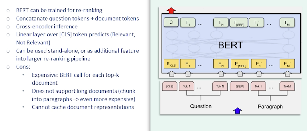
LambdaMART has proven to the IR community that machine learning can have tremendous impact in ranking. However these methods are only as good as the features you feed them. And so far we still haven’t discussed content features beyond just basic and ground match term frequency and documents frequency. These simplistic features do not allow for any semantic understanding therefore the search results will exhibit only a shallow emotional valence. In this class you’ve seen multiple groundbreaking advances and takes understanding based on large pre-trained language models for example BERT.

The question is whether BERT has similar models can be used to build search engines with more semantic understanding of user’s queries and the answer to that is yes. One way of doing that is to treat BERT as a re-ranking model in the re-ranking pipeline that we talked about earlier. To do that we would train BERT in a pair classification setup. So given a query document pair. BERT concatenate them and feeding into BERT and use the CLS token representation to predict the relevance level. In this way BERT can be used as a re-ranker just like any other classification model as covered earlier. The main rollback of doing this is that BERT is an especially expensive re-ranking model especially when scoring long pieces of texts. Therefore we need to think about latency carefully we need to chunk documents into smaller chunks if needed especially since we cannot reuse any document representation in the setup. We need to rerun the model for each new query.

Nevertheless large language models are powerful and people have gotten such setups to work with large gains in retrievable performance. So soon we will also look at how to leverage such language models for first-stage retrieval retrieving from a large collection of documents and not just in the re-ranking stage.

Embedding-based Retrieval, part 1

Ultimately information retrieval always is about efficiency and speed. We want to quickly search through billions maybe even trillions of documents and return results in an instant. Therefore running large machine learning models even for re-ranking has been a non-starter in many cases. And this is the main reason why the adoption of deep learning tools in information retrieval was quite slow. Ideally we want these models to be efficient scalable enough to be used in first stage retrieval but we still want to benefit from deeper semantic understanding capabilities of pre-trained language models. Towards this end we will now talk about embedding based retrieval.

First consider that we’ve already been representing documents as vectors as the columns and term-document incidence matrix. We talked about how this is a very sparse representation where only a very small fraction of the millions of possible terms will appear in a given single document. Similarly the term frequency and inverse document frequency matrices are also sparse vector representations of documents where the entries are real valued, rather than boolean.

We can do the same thing for the query as we’ve been implicitly doing when we talked about bag-of-words representations. And now suddenly we have two vectors in the same space which we can compare and calculate distance with. Ranking and retrieval then simply become a problem of vector similarity given the query vector which are the document vectors which are most similar to the query vector.

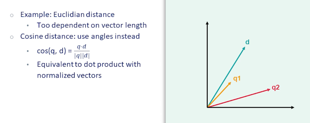
There are multiple choices available as far as vector distance functions. One common one is Euclidean distance. However this doesn’t work very well for retrieval because it is too dependent on vector length. For instance documents and queries with a lot of terms would have large vectors and therefore naturally large distance with almost any other vector even if they are semantically close. So cosine distance is another alternative which measures the cosine of the angle between two vectors. Cosine distance is equivalent to doing dot-product with normalized vectors so it’s independent of vector length. If you look at the figure here we have a document vector d in green and two query vectors q1 and q2. q1 is much closer to d and cosine distance whereas if you use Euclidean distance it wouldn’t be so clear which of the queries are closer.

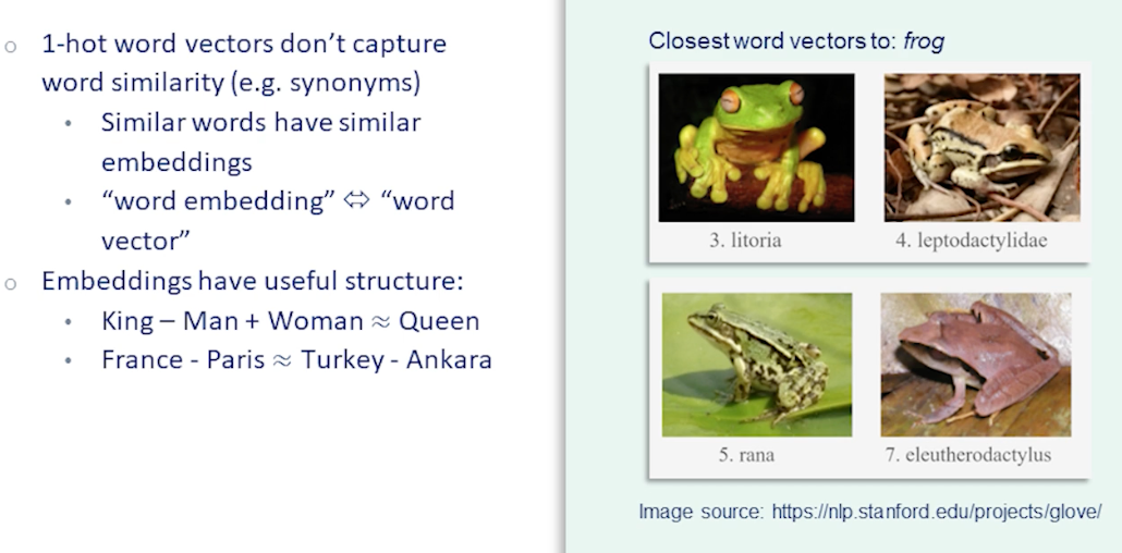
This brings us to embeddings.

Embedding of course is a vector and in fact the two terms are often used interchangeably. However embedding specifically refers to a dense and lower dimensional vector representation in contrast to the high dimensional sparse representations we were talking about so far. So why use embeddings instead of sparse vectors? Sparse vectors always have a lot going for them they’re precise they’re efficient.

Consider: the single-word query let’s say frog. So this corresponds to a one-hot vector which matches on that single term frog in the documents. However there are plenty of relevant documents talking about litorias or ranas or a thousand other types of frog which should show up in our search results. So these are after all also frogs. I heard this is very hard to capture with a sparse representation. So what we really need here is an embedding a dense semantic representation where a litoria a rana and a frog and the toads are presumably embedded close to each other in the vector space.

In addition embeddings tend to have useful structure. For instance if you take the embedding for the term king and subtract embedding for the term man and add “woman” instead you fall pretty close to the embedding for the word queen. It can also capture other relations such as “capital of” where France minus Paris and Turkey minus Ankara would roughly map to the same vector.

These similar properties can be useful for combining word embeddings to get meaningful query embeddings for retrieval.

Embeddings? Word2vec!

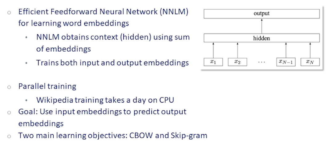
The early prototypica word embedding algorithm is word2vec which was covered in earlier lectures.

word2vec is trained by predicting a target word from the embeddings of neighboring words
We take a window around the target word
- sum their embeddings
- then feed it into a very simple feed forward network generating another entity

Given the target word embedding and a few randomly sample word embeddings

predict the target word from the output embedding
- by doing a dot product
- followed by a softmax
- and back-propagates on the error.

This simple algorithm is also very efficient and can be trained for example on the entire Wikipedia in under a day of CPU time on a machine.

So starting from this simple uncontextual word embeddings let’s see how we can build a very basic embedding based retrieval system.

To go from word embeddings to document and query embeddings

we can take an average or mean of their embeddings

$Q = \frac{1}{N_q} \sum_{i \in q} w_i$
- query embedding is just the sum of the embeddings of terms in the query normalized by query length
$D = \frac{1}{N_d}\sum_{i \in d}w_i$
- Similarly for document embeddings we normalize the sum of the embeddings by the document
then find the nearest document to query using a scoring function
- $f(d,q,w) = cos(Q,D)$

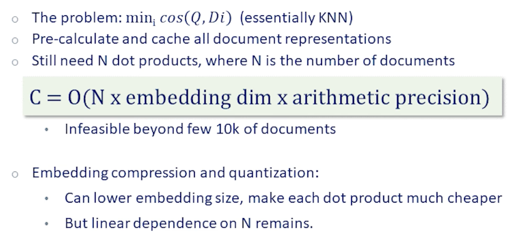
So we have nicely reduced retrieval problem into a k-nearest neighbors problem. The naive way to implement this is through matrix multiplication. If we assume for simplicity that vectors are normalized we take a dot product of the query vector each and every document vector and pick the closest one.

Clearly this would need N vector dot products if our documents correlation has N documents. Each of which needs d multiplications where d is the size of our embedding space. It’s possible to speed this up using embedding compression and quantization. However the linear dependence on the correlation size will remain. So this approach ends up being infeasible beyond a few tens of thousands of documents even if we pre-calculate and cache all of the document embeddings offline.

Recall that we ran into this very same issue when discussing binary retrieval. Naive approach of searching for query terms in each and every document proved to be infeasible and approaches which scale linearly with the document correlations size are simply not scalable in information retrieval since documents could number in the trillions.

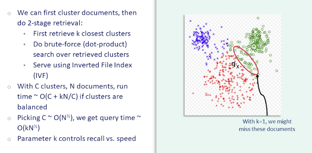
For term matching methods the solution was the inverted index which allows us to simply look up each term in the query and return documents containing that term which reduces the search space so we can return results in sublinear time. For fast embedding based retrieval we can use clustering to reduce the search space.

Suppose we divide our correlation into C clusters. Now we can do retrieval in two stages. In the first stage we find the k-closest clusters using their centroid embeddings. This should be fast since k should be small compared to the collection size. Then we consider only those documents belonging to these clusters and do brute-force k-nearest-neighbor search over those documents.

In fact we can now use an inverted index to serve this model. The cluster IDs replaced the terms to look up and the value returned would be the membership in the cluster which is the analog of the posting list. We call this the inverted file index or IVF method. Note that while the inverted index provide an exact implementation of term is retrieval IVF is not an exact implementation of nearest neighbor embedding search. There is a possibility that the top k clusters do not contain the documents we are looking for. For instance in this example figure we have three clusters of documents. Let’s take the case k equals we only look at the top cluster. If the query embedding happens to be close to the boundary between two clusters as in this figure then we’ll only look at one of these clusters the red clusters here. And we will miss all the documents in the green cluster even though those documents might actually be very close to the query embedding. Therefore fast embedding based retrieval with IVF is only approximate. However we can adjust the parameter k to arrive at a desirable accuracy-latency tradeoff.

With C clusters and N documents the runtime for this method is roughly O(C+kN/C). Since in the first stage there are C embeddings to consider and in the second stage there are k clusters each with roughly N/C documents assuming the clusters are balanced. If we pick the number of clusters to be proportional to the square root of N then the overall complexity comes out in the order of k times square root of N which is much better than linear. Combined with quantization this method can scale to billions or even trillions of documents.

Embedding-based Retrieval, part 2

In the previous section we described a working scalable embedding-based retrieval system. That basic system with mean pooled of word embeddings would do pretty poorly in practice. Let us look at several improvements that lead up to the use of modern pre-trained language model embeddings.

The first is DESM or dual-embedding space model, which is a minor variation on our basic retriever.

It uses normalized embeddings (instead of raw word vectors)
- $D = \frac{1}{N_d} \sum_{i\in d} \bar{w_i}, \bar{w_i} = \frac{w_i}{\lVert w_i \rVert}$
use different embeddings for query and document (recall in-out vecetors in word2vec)
- Mean of cosine distances (instead of the cosine of the avg embeddings)
- $DESM(d,q,w) = \frac{1}{N_q} \sum_{i \in q} \bar{D}^T_{OUT} \bar{w}_{IN,i}$

Aside from these minor differences DESM is similar to the simple retriever (BM25) we described earlier. And the results aren’t that much better. However, when both are combined with BM there is a slight improvement observed in the metrics.

The takeaway here is that term-matching methods like TF-IDF and BM25 though simple are very powerful and hard to beat.

The DSSM model short for deep semantic space model was another attempt for neural networks to break into IR.

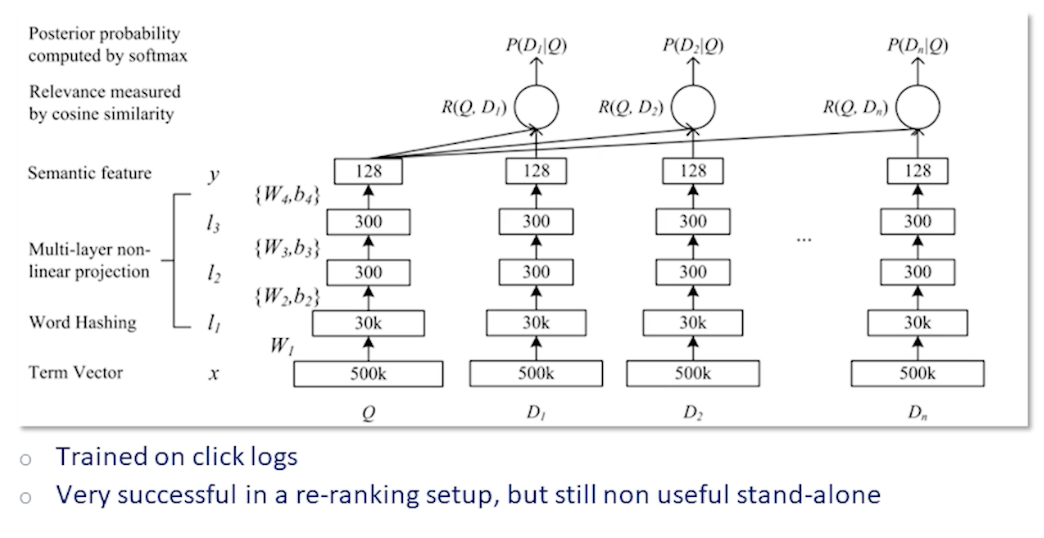
Here the sparse query and document vectors are first hashed into a smaller vector and then fed into a feed forward network. The output is an embedding of size 128. The relevance probabilities are calculated by taking cosine similarity of the query embedding with each of the document embeddings and computing a softmax. The model is trained on click logs providing labels for the softmax.

The DSSM model was actually very successful both in terms of research impact and in practice. Variations of this were deployed widely. However it was still only useful alongside a sparse retriever such as BM25. Its performance still not good enough to serve as a standalone retriever.

Which brings us to BERT. So we’ve seen in this course how language models pre-trained on large textual corpora have proven to be powerful tools for natural language understanding. Naturally the expectation was that the embeddings derived from BERT would also greatly improve IR. This did happen eventually however it took some work.

BERT embeddings out of the box actually perform quite poorly for retrieval presumably because they weren’t trained for that purpose. And training BERT for retrieval apparently needed a few more tricks. These tricks were outlined in a paper called dense passage retrieval which we will now go into.

Dense Passage Retrieval Paper

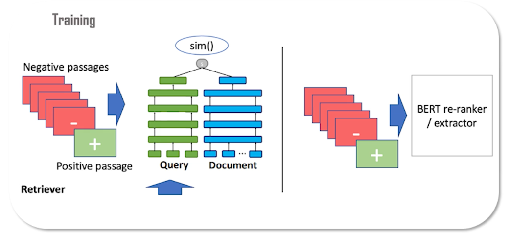
Here you see the overall architecture of the model.

The second stage you recognize as a BERT re-ranker which should be familiar from before. As discussed earlier the cross-encoder re-ranker is too expensive to use in the first stage. The first stage however is also a BERT model but in a bi-encoder setup. So this setup is similar to DSSM where two neural networks, one for the query and one for the documents, produce embeddings. At training time a training sample is composed of a query, a matching document, and a number of non-relevant documents called negative passages.

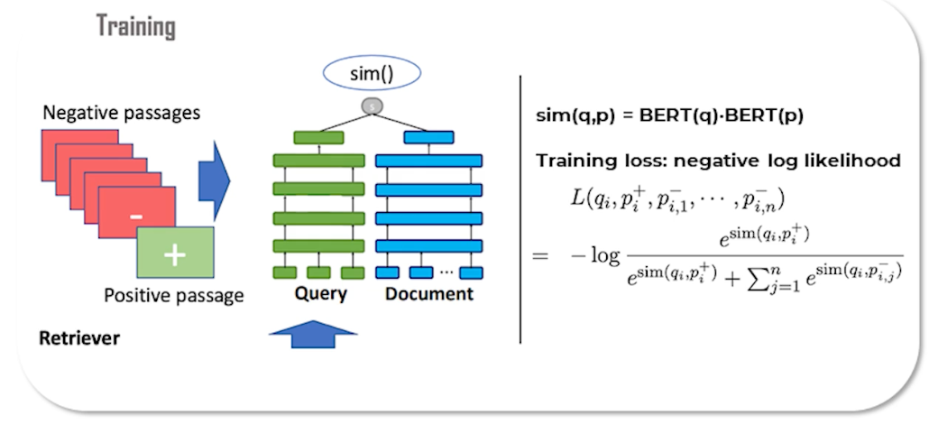
The query embedding is compared to each of the document embeddings through a similarity function which in this case is a simple dot product. Then we do a softmax and use the negative log likelihood loss to train the model. Both the query and document encoder networks are initialized by a BERT transformer model.

While training such a model it’s usually too easy for the model to tell apart a relevant document from random irrelevant documents. So even shallow term-matching heuristics are usually good enough. Therefore this baseline setup only provides a somewhat weak signal for learning. To improve we can introduce hard negatives into the training in the form of documents which seem relevant on the surface but are actually negatives. We can find such examples by using a baseline retriever system such as BM25. These negatives help the model converge faster and attain better accuracy.

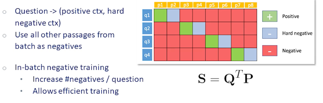
Running a large transformer model like BERT on multiple documents for each query during training can be slow. An efficiency trick is to take a batch of questions and reuse documents in the batch for all queries in the batch effectively increasing the number of negative samples by the batch size. This trick is called in-batch negatives and is illustrated at left.

For each question in the batch we have a positive document, one or more hard negative documents, and multiple random negative documents. Each query has its own positive document however the negative documents shown in red can be reused as negatives for every question in the batch. Since we calculate the document embeddings in the batch only once this effectively saves a lot of computation. In fact the positive documents and hard negative documents can also be reused as random negatives for the other queries in the batch.

We mentioned that these hard negative examples can be mined using an existing retriever such as BM25. It turns out that we can improve our model even further by getting it to train on even harder negatives. Where do we get these negatives? We get it from the dense retrieval model we just trained.

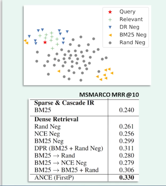
If you look at the figure on the right the query embedding is shown as the red star random documents are shown in gray. BM negatives which are the yellow triangles don’t actually look that much better than random negatives. However if you look at negatives obtained using a dense retriever model shown here in blue they’re much closer to relevant documents and therefore provide a more precise signal.

Thus training on negative examples mined using our last best model we can improve our model further. And we can keep iterating training on better and better negative exampes until the gains saturate. Finally I want to highlight some results from the table on this slide. The results are mean reciprocal rank on the MS MARCO dataset. The strong BM baseline achieves an MRR of on this dataset. The DPR model which is a bi-encoder BERT retriever trained using in-batch negatives and hard negatives from BM achieves a score of over 31 which is a full seven points over the BM baseline. So this is a huge improvement which finally justifies the use of large pre-trained models for retrieval. The ANCE model trained using harder negatives iteratively improves this even further to an MRR of 33.

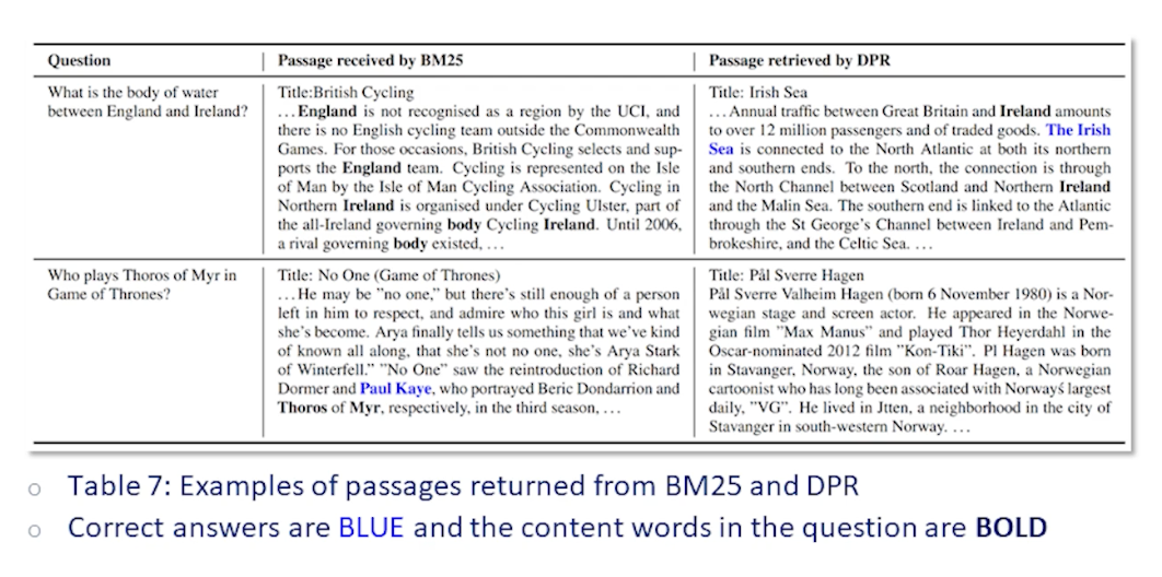
So the numbers are certainly impressive but let’s also look at a qualitative example.

Here we see two queries and compare the passages retrieved by the baseline BM system side by side with the dense retrieval result.

The first query is what is the body of water between England and Ireland? You can see that the BM return passage is heavily relying on term matching with the salient query terms such as England and Ireland appearing numerous times in the passage. Yet the answer to the question is not present in the passage. The DPR-retrieved passage on the other hand does answer the question. You can see the answer highlighted in blue. And clearly it does this by learning semantic relationships for instance matching England with Great Britain and relating the phrase body of water to mentions of sea and oceans in the text even though this passage is quite light on exact term matches with the query.

The second example shows a failure case for embedding based retrieval. The query here is who plays Thoros of Myr in Game of Thrones? But since the phrase Thoros of Myr is a very rare phrase the term matching system has no difficulty retrieving a relevant passage here which contains the answer.

On the other hand the embedding based system is not precise enough to exactly match this rare term, to exactly capture it in the embedding representation. This rare term it’s high likelihood never appears in the training data. So instead it retrieves another document on a similar topic.

So the preceding example highlights the complementary strengths of sparse and dense retrievers. Sparse retrievers such as BM are highly precise and they excel at term-matching. On the other hand dense retrievers capture more semantics therefore have higher recall but can miss some rare phrases where higher precision is required. In practice sparse and dense retrievers are usually deployed together in a hybrid setup to get the best of both worlds.

Another solution is training better embedding based retrievers. For instance we can use supervision from a sparse retriever such as BM to train a dense retriever effectively distilling that knowledge into the embeddings. We could also pre-train the retriever on large amounts of data increasing the coverage of rare words and phrases. Making embedding-based retrievers more precise general and robust continues to be an active and exciting research area. Thank you for listening to the lectures on information retrieval and see you in the coming lectures.

Module 8: Task-Oriented Dialogue (Meta AI)

Introduction to Task Oriented Assistants

In this section we discuss task-oriented dialogue systems. Task-oriented dialogue systems accomplish a goal described by the user in natural language. They often use pipeline approach.

The pipeline usually requires

natural language understanding for belief state tracking
dialogue management for designing which actions to take place based on the beliefs
and natural language generation for generating a response.

In this lecture we will go over:

introduction to the task-oriented dialogue systems
Intent Prediction
NLU and NLG Overview (Natural Language understanding NLU & generation NLG)
Dialogue State Tracking
Multi-tasking in task-Oriented
Error recovery in dialogue
Domain Knowledge Acquisition
Evaluation & Benchmarks
Open Problems

What is exactly a task-oriented dialogue system?

Well if one may want to understand user utterances to perform a task. Ex: providing information manipulation of objects navigating to a specific location. In case of house robot or social robot navigating to a specific location with voice commands could also be considered as a task-oriented dialogue.
Generating responses to user requests in a consistent and coherent manner while maintaining the dialogue history is essential for task-oriented dialogue systems.
While the user and system turns are effectively managed we could also see that recovering from these errors are actually an important caveat that a system needs to be aware of.
Engaging the user with adaptive and interesting conversations while progressing towards the common goal is also a key element for task-oriented dialogue systems.

Why is task-oriented dialogue a challenging problem?

Well the context of the dialogue history is extremely noisy and often it is important to keep track of the dialogue history to achieve the task success.
it’s also important for our task-oriented dialogue system to estimate the belief state of the user while resolving anaphora, repetition of a word or phrase, references during the discourse.
Piecing together all this information is necessary to complete this task.
domain specific nature of a dialogue can be very challenging and it will require some form of adaptation because lack of data or lack of coverage with different users. So generalization is pretty key for this problem. And you will see why soon.
API calls to web services could also change over time. And that will require frequent maintenance of the dialogue managers.

Task-oriented dialogues typically have three major characteristics.

Turn taking
- Usually dialogue is often interleaved between two speakers including the agent in this case or the system.
- each speaker would hold the floor for certain amount of time. they take the opportunity to speak or say something or inform something or request something to the interlocutor. And then the agent responds back depending on when the user has ended their turn.
Speech acts
- can be an important part of this understanding of the dialog system.
- assertives are essentially to say the speaker actually suggests are put forward some information to the agent.
- directives can be very different from assertives where they just ask or request information.
- similarly commissives are speakers. Actually speaker is agreeing or opposing the agent so they say yes or no.
- expressiveness is as simple as saying hello or goodbye.
Grounding
- whether the user and the agent usually agreed and have a set of information exchange
- the agent actually acknowledged the user’s exchange information.

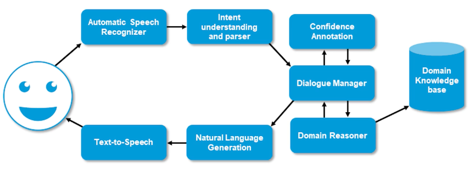
Above is an overview of a typical task-oriented dialogue system architecture or pipeline. So when you have a speaker and he or she would say in actions and the automatic speech recognition system would recognize their options and finally run it through an intent understanding and a semantic parser which fragment the utterance into necessary components where the system could understand and it is sent to the dialogue manager which orchestrates the entire conversation history and context. And which actually interacts with the domain reasoner which basically interacts with a knowledge base or a database which is essential for providing information to the user. And then once the information is back from the domain knowledge base or a database constructive response using natural language generation module which is further sent out to a text-to-speech engine which basically synthesizes the system response in a speech form.

There are several terms that we’ll be using in this lecture. And some of the important terms are domain intents and slots.

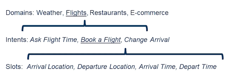
domains: can be weather, flights, restaurants, or e-commerce
intents: are classes that a user may initiate in a given domain. ie flight time, booking a flight or change of arrival
slots: are basically the entities or spans that are contained in a given utterance which would essentially lead us to a certain intent.
- For example: book a flight intent
- would require arrival location, departure location, arrival time, and departure time.

Automatic Speech Recognition

This segment is an overview of speech recognition natural language understanding, NLU, and natural language generation, NLG.

Automatic speech recognition systems are often used in understanding user speech. These user utterances are often required to be endpointed for speech segments alone because they may also include silences as well.
Acoustic features are computed on these endpointed user utterances This means essentially we’re looking to translating these raw acoustic features to some phonemic sequence which is an approximation of how the user has produced relevant syllables in a given language.
this phonemic representation could be further translated into subwords or full words and conditioned by the language model.

Acoustic models are typically used in order to discriminate between certain phonemes how the speakers actually pronounce certain things

Acoustic Features: Traditionally mel-frequency cepstral coefficient
- whether the acoustic features represent certain phonemes or not
  - this can be done in two ways
Acoustic Model - two different ways:
- Discriminative model either speaker dependent or speaker independent
- To realize the phoneme / subphone sequences on the acoustic features
then you apply a Lexicon or a pronunciation model based on a statistical information in a given language
- how the syllables are constructed
- which in turn can be realized further into words or tokens in a given language
The language model
- provide the token-level transitional information
- which token proceeds which token and so on and so forth

Often in this setting you also have certain slot values.

Slot values are specifically named entities or spans of tokens that are useful for providing information
these slot values could potentially be out of vocabulary at times
- if the users are requesting information that is potentially outside the domain or outside of the knowledge base that the system is trained word.
the ASR challenges in this situation are pretty intense
- because often the conversational speech and conversational speech is very different from a typical dictation or voice-based search.
- So acoustic models and language models may require large amounts of data in order to address their switches where they’re potentially likely to fail.
ASR models in this situation often are evaluated on word error rate or Character Error Rate metrics
In task-oriented dialogue setting slot error rate is more applicable that captures the errors and important information in a given speech hypothesis.

Natural Language Understanding

Natural language understanding is composed of multiple steps, but sometimes it could be done in a joint modeling way.

let’s look into the details of intent prediction. It refers to extraction of semantics from the natural language utterance that a user has uttered to determine the user goal during the dialogue.
Then converting the speech recognition output to a semantic representation often involves lot of challenging situations such as
- ASR errors could occur specifically in the slot positions where the words could be mangled around which potentially could cause misunderstanding of the user utterance.
- ambiguity is also another issue.
- synonyms appear often human language , multiple meanings,
  - this can cause same word being misinterpreted in different ways.

Natural language understanding typically has three phases

intent prediction ( primarily goal is understanding which is information seeking or clarification )
slot filling (slots relevant to the task/inputs needed to complete the task)
state tracking ( maintaining a distribution of slot values and how the user conversation has progressed )

Slot filling in this case could look into the example here.

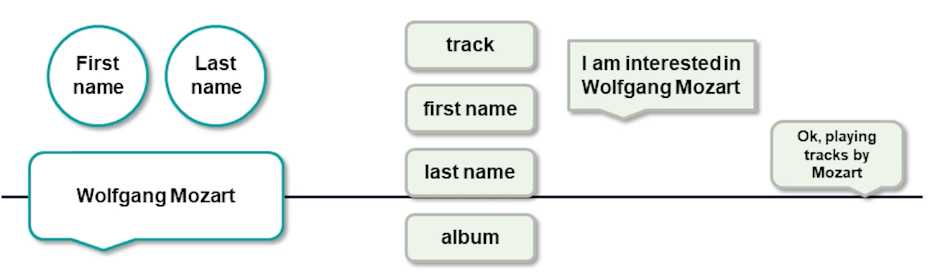
I’m interested in Wolfgang Mozart. let’s say it’s a music recommendation system. And you basically have defined slots as a track or the first name and the last name of the artists and the album name. You can see that the first name and the last name of the artist is captured by the system. Optionally the album or the track name could also be captured if the utterance includes it. In this case it doesn’t so we simply go on to okay playing tracks by the Mozart and so the system has addressed the user’s request.

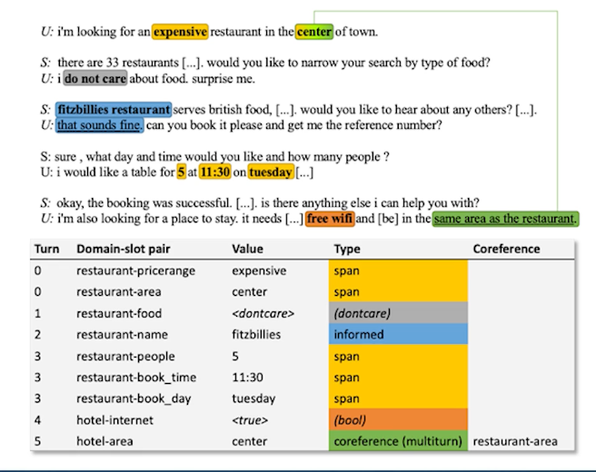
Here is a more complex example where you are actually looking for a restaurant in a certain place. And this is an example from the Cambridge Restaurant Information System which is deployed in real life situation.

user asks: I’m looking for an expensive restaurant in the centre of town
- system responds: There are 33 restaurants
to narrow down the search it cares about if the user actually needs certain type of cuisine
- then the user responds back. They don’t care about specific cuisine
Then the system gets back it takes a turn
- then says some restaurant which serves a certain particular cuisine.
- the user is interested in the restaurant and asks the system to reserve a table.
- the system responds back with the time and number of people who would like to be assigned to the reservation.
- User follows up with that and the system actually books the reservation successfully and user follows up with an interesting request here which actually one would note that this is a multi-domain dialogue system. The reason being the user is asking for a place to stay which is a hotel reservation which is I would envision the system and as a multi-domain task oriented system because it requires a different set of slots it requires different set of understanding modules. The system accomplishes that task apparently.
- As you can see the hotel area in this case is referring to the same area as the restaurant which is a conference resolution that needs to be performed by the system in order to achieve the second task.
- The natural language understanding in principle involves several complex interaction between modules. We’ll look into the details of it furthermore in the slides.

Natural Language Generation

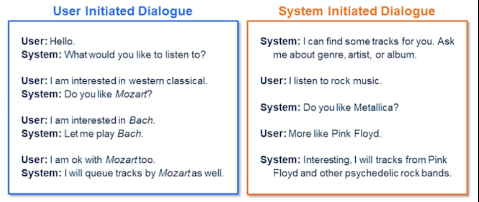
Natural language generation usually can take two forms: User and System initiated dialogue. Let’s walk through these couple of examples in front of us.

In the user initiated setting the user drives the conversation.

And as you can see the user has asked requests about Western classical music and the system response back whether they like Mozart and the user responds they like Bach. And the system will oblige the request and also the user makes a correction to his previous request saying but they also like Mozart. And the system replies back saying they will queue and queue tracks from Mozart as well.

In this conversation the system always takes a backseat and tries to acknowledge the user’s questions or confirmations. And based on that it does provide information or performs a request. In this case like adding music to the playlist.

So in the system initiative dialogue on the right hand side as you can see the system is more capable of providing array of potential requests that a user could ask. And this way the system has more control over how the conversation can be driven. So certainly it can avoid out of domain request not necessarily all the time but for most part because it’s a user is aware of what the system is capable of as opposed to an end user initiated dialogue. So you can see that system preferably drives the conversation by asking whether the user could provide a genre artists or an album. And the user has given in this case the genre information and also an artist information in this case.

Task Oriented Dialogue

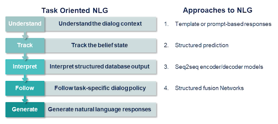
Task-oriented dialogue typically has 4-5 different states.

first is understanding that dialogue context. The dialogue context meaning whatever the dialogue manager has previously provided or the previous conversation previous turns etc
the belief state which is essentially what slots have been fielded and how the user has been going on with the conversation. Are they happy with the conversation or not?
interpreting the structure database output which is essentially once the information is considered from the domain reason or our database.
Now the system has to respond in a structured fashion using a dialogue policy. A dialogue policy enables the system to answer questions in certain ways. So whether it has to be crisp answers or they can be more elaborate depending on the dialogue state or the number of turns that have passed through during the dialogue.
finally the generating the response and a national language fashion which either take the forms of template or a structure prediction form where you essentially have a semantic structure that maps back to a free-form natural language.

More recently people have been using sequence to sequence and encoder-decoder models in order to achieve the same and structure fusion networks are also popular methods to achieve task-oriented dialogue generation or natural language generation.

Here’s an example of restaurant domain dialogue natural language generation.

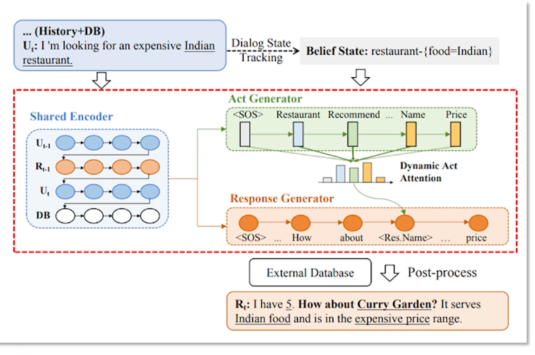
As you can see the user at time t have something I’m looking for an expensive Indian restaurant. And in this case the system is already kept track of the previous dialogue history and also the database responses. So once the dialogue state tracking has updated than the belief state in this case the restaurant of interest is of type Indian. And the act generation part which is let’s assume it’s a neural network that basically a process which restaurant names to be added into the slots the names and the prices etc.

finally the response generation takes over on the actually manifesting the real response. So in this case you have seen that as a shared encoder which basically has the previous user history such as previous term in this case t-1. And what was the system response and the new user turns context. And also finally the database. Along with this information the system is also capable of providing a slot level attention. So that way it has a sense of which information needs to be more critically captured and where the mistakes can not happen. So in this case let’s say the name of the restaurant cannot be wrong at all or it has to be in the vicinity of the user. Let’s say and or in this case the criteria is that it has to be an expensive restaurant. So that adds up to the critical part of the response. Finally the system responds back saying I have five and our Curry Garden it serves Indian food and hence the expensive price range. It could also be other constraints such as the location need to be within the range of two miles or one mile and so on and so forth.

Dialogue Manager

Let’s turn our attention to how a dialogue manager functions.

A dialogue manager typically orchestrates the content and structure of the dialogue

process the input from speech recognition and natural-language understanding modules
track the history and the context of the dialogue in the form of a state
exchanges information back-and-forth with the domain reasoner, to get the data back for the user
then broadcast it to the user via natural-language generation in speech synthesis
Dialogue managers often use data structure for storing the context and the task relevant information.
Dialogue state tracking is a mechanism to update this data structure so that the user would ultimately succeed in their goals.

A dialogue management can achieve this by constructing a task tree. So typically a dialogue system developer would construct this task tree using

a finite state automaton as simple as handcrafted character dialogue task tree with fixed transitions between dialogue states.
System typically initiates the dialogue and controls the flow in a very rigid fashion based on series of questions could be very well like a questions game.
System may have difficulty sometimes to recover from non-understanding errors in this case.
this is good for small and limited domain dialogue systems so that you could rapidly prototype and how the dialogue users would experience the system.
A good example of this mechanism is VoiceXML.

And often dialogue management is through frames used by the data structure typically

Slots and slot types are filled based on the questions posed to the user
- ie restaurant name, reservation time, cuisine type
Slot types are often hierarchical in nature where the slots are included in these frames.
- Thus complex dialogues are performed via tree like dialogue state transitions
- And you typically see slots and slot types are fail based on the questions.
This allows multiple domains and multi-intent dialogues with slots tied to an intent.

Dialogue tracking typically consists of processing the user requests and then information and filling in the slot while keeping track of the user preferences, which could be prior information and so forth.

There are handcrafted base systems to track the dialogue state.
Or there are also probabilistic based methods where you maintain the distribution of the values per slot.

Dialogue policy typically the mechanism how the actions can be performed what actions can be performed by a system given the dialogue contexts in the state.

So every system action can be determined either by a handcrafted or a train policy given the dialogue history. And handcrafted in this case could be as simple as like we discussed VoiceXML based like flowchart etc or
the statistical one which are more sophisticated use reinforcement learning or partially observed Markov decision processes.

End-to-End Task-Oriented Dialogue

Let’s now look at an end-to-end task-oriented dialogue system, with a primary focus on how different modules discussed earlier would come together.

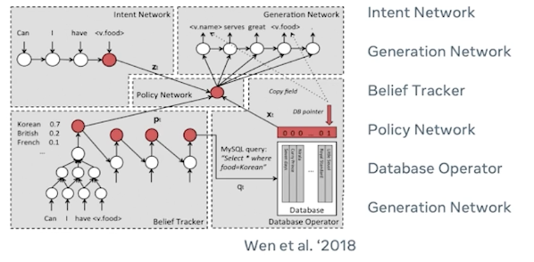
Let’s imagine this architecture proposed by Wen et al in where you can see there are multiple deep neural networks that are involved in orchestrating different mechanisms in different phases of the user actions. So there are primarily six or seven different networks involved in this case so we’ll deep dive into each one of them briefly look into how they operate.

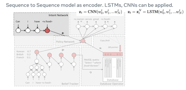
First one is intent network where we see the sequence-to-sequence model. In this case could be applied where it could be an LSTM or a CNN or for that matter any sequence-to-sequence model which would basically consider the user’s utterance delexicalize it. So when I say delexicalization you’re essentially masking out the user’s intent or the user’s actual utterance with a typical slot value in this case the <v.food> is basically the value of the food type that is being masked out. And in this case the user’s utterance could be can I have Indian food or can I have tacos? So that could be an utterance and then it gets masked out by their relevant slot type.

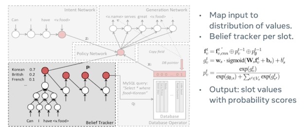
the next step is belief tracking where the belief tracking maps this input to distribution of values so it can keep track of various different values. And often the belief tracker operates per slot. So let’s assume in this case it’s looking at the cuisine so let’s see. We can see that Korean is assigned 0.7, British is 0.2, French 0.1. and so on and so forth. And finally the output is slot values with probability scores assigned to it like we discussed.

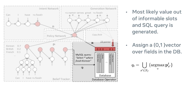
In this setting typically a database operator may fetch multiple values depending on the slot value. So again these restaurants could also be assigned certain values certain probability or a certain way to optimize for user’s preferences. So one would say let’s try to apply an argmax or to optimize for users’ preferences and their needs as expressed in the request. And MySQL query could typically look like this like “select * where food = Korean. this would essentially bring back all the values that are unique in nature and then sent out to the next step.

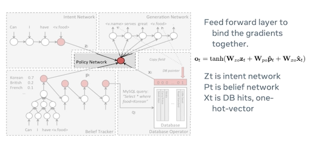
There is a policy network which sits in the middle and binds all the different modules. It’s typically a feedforward layer to bind the gradients together. And you would see that Zt in this case is the intent work and Pt is basically the belief network in the equation. And Xt is the database hits which is basically that is a list of Korean restaurants in their one hard encoded form.

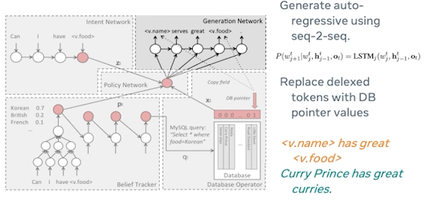
Next we see the generation network is responsible for generating the actual response to this user. In this case it’s again a sequence-to-sequence method which is basically replacing the delexicalized tokens with a database point of values. So I told earlier that in the intent network phase we basically delexicalized what the user is intending at in order to capture their intent using the train models and that will actually help the database to figure out which are the pose potential values that we can include. And this is where replacing the delexicalized tokens with the database pointers would help in generating a valid response.

Model Training

Training belief networks between wizard and belief distributions can be challenging. Training end-to-end using these systems which requires some form of a visitor wall setting or wizard sentences that is like a human actually pretending to be a system and generating their response to a given user’s request. So often that dataset would help us rapidly evaluate a new leader train models in this kind of a setting.

Decoding

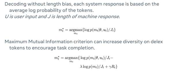
At the decoding time often you decode without length bias so that you can have different lens of different responses so that you’ve introduced certain diversity in the response and the variability in the response. And often sometimes the restaurant names could be longer and so on and so forth.

So each system response can be based on average log probability of the tokens

this helps to control for the machine’s response so we don’t over-generate text.
it also allows sometimes the downstream speech synthesis system also be able to say that exact word the way it was intended to be. Otherwise the user would not understand the system’s response even if the system response was correct.

Another method to generate these responses or decode responses is MMI

Maximum Mutual Information criterion can increase the diversity on delexicalized tokens to increase task completion.

Belief Tracker Performance

So if we look into the belief tracker performance often the belief tracker which captures the slot values information and places them into distribution one might claim that precision is most important. But while the precision is important which actually measures how accurately we understood the user’s request in the first place it’s also important to look into the recall in this case which is the information that was returned by the database and followed up by the response generation is also accurate enough. So that is basically providing how likely the user would accept the response or the restaurant information from the system in this case.

Interleaving Between Different Related Tasks

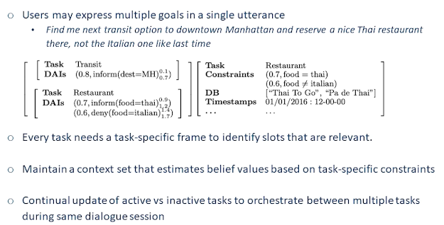
As we are talking about multi-domain in one of the earlier slides it’s important that the systems often make sure that when the user has requested for multiple tasks in the same utterance so in this case one may consider this example find me next transit option to downtown Manhattan and reserve a nice Thai restaurant there and not the Italian one like last time. So this had several things to unpack. So there are at least three tasks involved.

there is a transit task involved where the system has to figure out where the user is like to head to
then find a restaurant in that particular area. So that’s a second task.
in the third task they wanted a restaurant that was not based on their previous preferences.

So they wanted something else not the Italian food. So I think this also involves keeping track of across the session a contextual history which can be extremely challenging for a system to call back into certain past history and then figure out this is not what the user wanted. So this is where the user preferences come into play. And there are more sophisticated systems to solve this setting where this setting we will not go into the details of it but we’d like to just present this as a situation or a dialogue system could potentially face. And in this case every task needs a task-specific frame to identify slots that are relevant and maintain a context so that estimated belief values based on the task-specific constraints. And it also requires continual update of active and inactive tasks to orchestrate between these multiple tasks in a given dialogue session. So one may see that transit task is performed then it becomes an inactive task. And then now finding out the restaurant is probably more important while keeping track of the user preferences.

Error Recovery in Dialogue

As we move further into the dialogue system stack we see that errors will obviously naturally co-occur in this kind of a setting where you have multiple tasks or even with a single task dialogue system.

So there are two kinds of errors often occur. misunderstanding and non-understanding error.

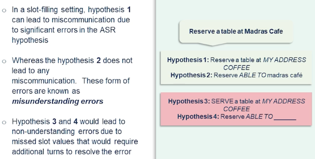
Misunderstanding errors often occur due to the speech recognition errors that occur in some form of recognition errors that can not be recovered in that particular instance but could be recovered from in a follow-up patterns. So in this case it is something like the hypothesis .

From the speech recognition, it looks like this.

There’s our table at My address coffee
was miss recognized “My Address Coffee”. And that could be recognized.

The rest of the utterance was recognized correctly except the named entity in this case “My Address Coffee”. So this may lead to some miscommunication but does not really derail the dialogue.

Whereas the hypothesis doesn’t even derail the dialogue because it got all the relevant slot values. And this is where slot rate like we discussed earlier when we were discussing the ASR evaluation one would say okay the slot was correct so it's actually % accurate. Whereas in the further down the list we see hypothesis and which lead to non-understanding errors due to missed slot values. And that will definitely require additional terms to resolve the error where the utterance does not really provide any information about what the user is intending to say.

Often there are three different recovering strategies from failed dialogue options, dialogue misunderstanding, etc.

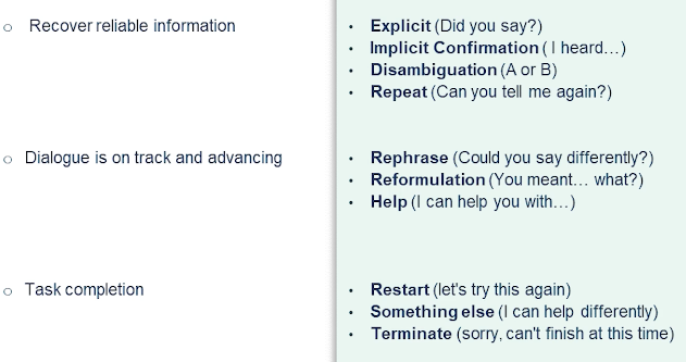
So first one is recovering reliable information.
- by explicitly asking did you say or implicitly confirming I heard you say disambiguation.
- Do you want A or do you want B?
- Basically providing envious list options but just restricting it to two.
you could also how the system ask the user repeat can you tell me again whatever you have said in the previous sections? And that’s what obviously upset the user if it has been happening repeatedly. But it would be okay just to use that strategy once in a while. And dialogue is often something that needs to be tracked and whether you need to look into whether it’s advancing or not.
- rephrasing the formulation and providing explicit help what the system could actually do is super relevant and important.
Finally task completion require some times restarting the dialog altogether. And sometimes you just have to terminate the dialogue because the user satisfaction cannot be achieved. And it’ll potentially reduce credibility of the system altogether.

Evaluation and Benchmarks

Dialogue Evaluation Metrics

Overall empirical metrics typically include
- task success, Number of dialogue turns, slot error rate/accuracy
NLU Evaluation can be further broken down
- Slot-level F1, Intent prediction accuracy
- Belief state or dialogue state rewards
  - provide feedback to the system
NLG Evaluation also has some nuances such as
- BLEU, METEOR scores measure human response against reference
- Slot error rate or information accuracy towards goal completion
  - how satisfied is the user?
Human ratings such as Likert scale, single-turn or multi-turn evaluation are more suitable for overall interaction quality
Multi reference evaluations often require denoising of ratings, and higher inter-annotator agreement
- People may or may not judge the conversations in the same light. Some might be more tolerant than the others.
Recent work on DialoGPT proposed a FED metric that automatically measures the likelihood of generating positive/negative follow-ups for a given system utterance. These metrics would often help guide the user or the developer I would say to actually build dialogue systems that can be rapidly prototyped for a given domain.

Task Oriented Dialogue Datasets

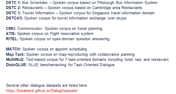
Dialogue Benchmark results

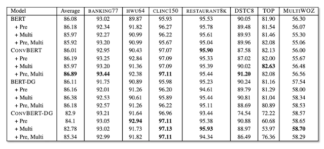
Tongue of DialoGLUE which actually is one of the largest benchmarking platforms for the task-oriented dialogue it includes several datasets such as banking which contains about utterances related to banking with nearly different fine-grained maintains. Clinic it is another kind which spans about 10 domains with different classes. That is HWU64 which includes intents patents spanning domains including alarm music IoT news calendar etc. That is Restaurant K dataset which comprises about notions as it clearly says in the name. And the DSTC8 is one of the state tracking data sets consists of slot annotations spanning four domains. And so this is actually the DialoGLUE includes several benchmarking methods such as the BERT base convert which is basically BERT trained on open domain dialogues. And BERT-DG which is a BERT trained on full dialogue load data in a self-supervised manner. That is convBERT-DG which is convert trained on full dialog flow dataset.

Like I said as you can see in the experimental results one may see the fine-tuning. The BERT on large open datasets like DialoGLUE could essentially produce a pretty decent model such as convert. And in this case actually one way find this task after training is one of the key components especially when you are looking into dataset-specific findings. So what we’re really looking at in this case is sometimes you may fine tune a given pre-trained model to a target task. However fine-tuning on a specific dataset task may not really yield a better results on other datasets even though they may look similar in terms of the spirit of the domain. And that was one of the findings from this particular benchmarking efforts in DialoGLUE.

The performance gains due to the task adaptive nature is more often promising than actually doing a pre-training on the open domain dialogue dataset altogether. Self-supervised training on the same datasets obviously help in a few short learning setting. And this is well understood in other machine learning tasks. this is a promising direction as well for the task-oriented dialogue systems.

Challenges and takeaways

In the end we can look into some of the challenges that we have discussed over the last several slides and some takeaways here. Task-oriented dialogue is often challenging just because the sheer scale and limitations of the domain-specific datasets and sometimes the scale of the dataset may not match the number of users or the other way round. And the conversational speech recognition is an active area of research which is I would say is not covered in this talk but should be a very promising direction first task-oriented dialogue especially when we need to understand what the users are saying in different dialects and likely to use different named entities etc. Ambiguity in understanding language can be pretty noisy and the natural language understanding systems need to work hand in hand with the speech recognizer in order to perform better. We have seen that sequence-to-sequence approaches have shown some promise in this direction and ability to generate natural and engaging responses have been promising but we’re yet to keep track of the slot-level accuracy.

So over generating texts can be pretty challenging and can be detrimental for the understanding of the user because if it were a robot trying to understand an utterance and then respond back to the user in a very over generated texts then it’s unlikely that the user would understand whether the robot has performed the action or not. So dialogue state tracking is also particularly a key area which is covered several times in several data sets like DSTC see datasets are primarily targeted in that area. So there are several approaches that addresses this problem in more details.

Module 9: Applications Summarization (Meta AI)

What is Summarization?

What is summarization? (use cases and different ways of summarization)
Metrics and Benchmarks
Neural Models for Summarization
Pretrained (Neural) Models for Summarization

What is summarization?

There is a lot of information that is floating around: Online, personal life, emails, text messages etc etc
A good summarization system faithfully present only the most relevant information that is needed
- What emails should be on top?
- inside each email what is it that I need to know and what is it that I need to respond to?
- news articles usually have their main bullets at the top
Consider the sentence
- Morocco have beaten Spain on penalty kicks and will play either Portugal or Switzerland for a place in the semi-finals of the 2022 World Cup in Qatar
What makes a good summary?
- faithfulness: the system is not making things up. It’s true to the facts it’s not adding or changing the facts.
  - ex Morrocco beat Spain vs Spain beat Morrocco (unfatihful)
  - both have very different meanings but use the exact same words to summarize
- Relevance: system has to capture the most informative part that I need
  - Morocco appeared in the World Cup
  - this is faithful but is it the most relevant piece of information?? Probably not
- coherence and cohesiveness
  - there is a slight difference between the two
  - coherent sentences have to be telling a smooth story.
    - ex: Morocco beaten Spain play either Portugal or Switzerland
    - Is rather poor english, despite being relevant and faithful
  - cohesive sentences have to be aligned and be related to each other
  - This again depends on the context and level of formality and the mode of a dialect of language you use. But if we stick to for now we’ll look at proper English this sentence is not proper English and it has problems in terms of coherence.

Extractive vs. Abstractive Summarization

And here we are going to be diving into different ways of summarization.

Consider the sentence: Morocco have beaten Spain on penalty kicks and will play either Portugal or Switzerland for a place in the semi-finals of the 2022 World Cup in Qatar

There are two main ways of summarizing a sentence or a document.

Extractive
- Some of the original sentences (or sub-sentences) are picked as the summary
  - use or reuse the original sentences and treat them as a summary
- Pros: Guaranteed to be faithful
- Cons: it can be redundant and may lack coherence
  - often removes some context and might change meaning or just drop a word that would negate the meaning might also result in redundancy if the sentences picked repeat each other’s theme
  - “Morocco have beaten Spain on penalty kicks
  - Extractive approach is done a lot with news articles, and works relatively well for that domain
Abstractive
- Generate the summary from scratch.
  - This resembles what humans might do. we just pick and choose and we change words as needed.
  - We bring fillers and connectors and make a smooth summary.
- Pros: Summaries are generally coherent and grammatical
  - especially if you use a good language model for your decoder
- Cons: Faithfulness can be an issue ( hallucination )
  - hullicination refers to the event that the model could just bring something up or make something up that just never happened and it might be even factually correct.
  - this can happen when using pretrained models.
  - ie the model have a lot of info about Portugal that comes out in the summary, but isn’t part of the document being looked at, or part of the subject matter
- Morocco beat Spain in the Qatar world cup
Extractive/Abstractive
- a combination of the two methods (useful for long documents)
- you can’t put everything in memory sometimes.
  - first extract some pieces of the document that you think are the most relevant. reduce down to say 1-2 pages
  - once you do that then you can give it to an abstractive model
  - your output from the abstractive model
  - is something abstractive and concise and lacks redundancies

Summarization Evaluation

Methods to evaluate the summarization task.

generative task are pretty hard to evaluate.
generative tasks include: translation, summarization, and data to text
- Summarization can be difficult, as the space of acceptable summaries can be large

Data to text usually refers to a problem that you have a knowledge graph in terms of triples. And you have bunch of triple facts and you want to put them into natural text and glue those facts together. These tasks are hard because to evaluate because the space of candidates are vast.

And it’s unlike the discriminative tasks such as classification task that you have the label and you have good metrics like F score. And you can measure if your predicted label is correct or not. And you have f mod metric and you’re pretty good. For a lot of task even you have multiple references that you can compare with but it’s still it’s not exhaustive. And even if that’s you’re close to one of the references it’s not immediately obvious if your candidate is good or not. For example. it could have changed one word that would change the meaning of the whole thing. So that’s why that these tasks are much harder to validate than classification tasks.

In summarization especially this is an issue that makes even things trickier because this space of acceptable summaries or even larger than what you get from translation. In translation you’re really poke candy. Original document or sentence that you’re translating. And you have to basically everything you can pick which part of the centers you want to translate. But in summarization you have that element of retrieval that which part of the article you want to focus on. And then once you know which part do you want to be focusing on how do you present it? And so that’s why there are a lot of problems could happen in either of those steps. Those steps could be happening implicitly like an abstractive summarization but it’s still they’re all up you can imagine pipeline.

Faithfulness is hard to measure
- Same words different ordering can make it unfaithful
Relevance can be subjective
- Morrocco beat Spain on penalty kicks
- Morocco beat Spain to reach the quarter finals

Now depending on which one of these facts were mentioned in the reference summary you could be penalized hugely even though both of these are probably good summaries. There are many automatic metrics for summarization and generative task in general. But at the end of the day especially if you want to deploy a system human evaluation is inevitable that how good your summaries are especially interpreter faithfulness that relevance is still is pretty subjective. You can be lenient about it but faithfulness is something that it’s a big no-no to make when you want to make a system deploy.

So here we’re going to be talking about ROUGE, but first let’s do a quick review of BLEU.

EvalMetric-BLEU

measure of the precision of the translation compare with the original reference translation
Brevity Penalty is added to penalize it to not be super short and super precise
Hard to interpret: N-gram match for several n altogether
- that we have one metric for all the n-grams
- whatever n-gram that you choose everything is mixed together
- and it spits out just one metric

Some of these issues will be resolved by ROUGE

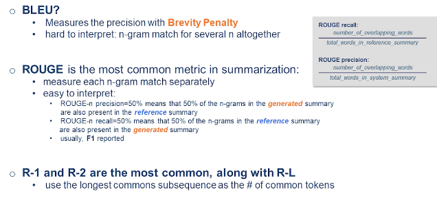
EvalMetric-ROUGE

Is the most common metric in summarization
Measure/treat each n-gram match seperately
easy to interpret
- ROUGE_precision = num_OverlappingWords / totalwords_inSystemSummary
  - looks at the number of overlapping n-grams
- ROUGE-n precision=50%
  - means that 50% of the n-grams in the generated summary are also present in the reference summary
- ROUGE_recall = num_OverlappingWords / totalwords_inReferenceSummary
  - representing as many as possible the terms in the original reference summary
- ROUGE-n recall=50%
- means that 50% of the n-grams in the reference summary are also present in the generated summary
you often see these called R-1, R-2, etc etc
- the number refers to the n in n-gram that it is looking at
- R-1, R-2, are the most common
Another common measure is the rouge score R-L which it uses the longest common subsequence between the reference and the predicted summary. Instead of overlapping unigrams or bigrams
- Usually for when you have a summarization system that is better than the other one it all this R1 R2 RL can be better than the other one. But sometimes some of them capture different effects.

Problems with ROUGE

The biggest problem with ROUGE is that it only looks at tokens and token match and doesn’t consider the semantics.
There are some versions of it that look at the stem of the word and won’t penalize for variations
- for example: work and working.
- But a different word with the same semantics might be penalized
Another problem that comes up is that a candidate could be completely wrong and has factual errors. But might get high ROUGE scores if it has enough overlap with the reference. So you can throw out the words and bigrams or whatever and still get a high score. Or that’s what RL can penalize those stuff. But it still is not enough. You could have a huge overlap at the beginning and while the rest of it is nonsensical it’s still gets big RL and as well as the other R1, and R2 but just be nonsensical summary.
the last problem with ROUGE is that it ignores the original document. So you have a reference summary or multiple reference summaries if you use a good dataset if you have those usually you don’t just have one reference summary for the whole article. And you’re calculating and evaluating your system based on one single or multiple candidates can references. So there could be a lot of valid summaries.

there are some metrics that have been introduced to counter some of these limitations.

the first one that was introduced in was BERT-score.
- This looks to mitigate the limitation that ROUGE doesn’t consider the semantics.
- here instead of looking at the word overlap we give both the reference summary as well as the predicted one to pre-trained encoder like BERT.
- then we look at the contextualized embedding for each of them
- And we look at the cosine similarity between the candidate and the reference
the latest one in that was introduced is BART-score.
- In BART-score you use a BART model (a pretrained seek-to-seek model) to calculate the probability of the summary candidates given the original documents. So here you use the original document in the formulation as well. For this BART-score has multiple variants.
- in some of them it would use the original document as the source and try to calculate the probability of the target which is the predicted summary. this usually is good measure of faithfulness. That if you are making things up in the predicted summary that probability is going to be low that you have introduced new facts original document or change them.
- The other variation is to look at the reference summary as the source and the target is a predicted one again. Similar to how ROUGE or BERT-score with work. And we’d look at some irrelevance of how relevant your summary is compared with the reference once.

BART is one of the few metrics that we have to measure faithfulness. Because in a faithful metric you have to consider the original document.

Benchmarks

here I’ve listed some of the benchmarks and you will see on the papers usually.

Historically summarization was first introduced and super popular for news articles. And it still is being used a lot in most of the websites, such as CNN, Daily Mail, New York Times is probably the most common summarization task and dataset that you will see in papers. And it’s a pretty extractive dataset like most of the news articles.
- For all of these the summary can be pretty much be written from the words that exist in the article and sub sentences or even full sentences. for example a good baseline for all those datasets is the top three sentences. And it’s a non-trivial baseline to beat.
XSUM is on the other side of the spectrum.
- It is probably the most popular abstractive summarization dataset.
- here you have a short article bunch of sentences not as long as CNN but it’s still pretty long. And you’ll give pretty much like the title for it. So you can think of it as a news article title link task which is a much harder task than the CNN Daily Mail and harder to evaluate as well.
Recently there are a lot of multi-document datasets like Multi-News
- here you have multiple news articles that you want to summarize together.

And the other aspect of this task this long summarization that we mentioned in the section on abstractive methods.

here you find ArXiv papers and PubMed articles used to evaluate those systems.

There are standard summarization tasks as well though not as popular as articles. This has its own field of methods and stuff. And usually GigaWord is a good dataset for that. For here as it’s pretty obvious is that you have a sentence instead of an article that you want to summarize. And sentence simplification is something that is pretty close to this test as well.

There is also some niche articles and there’s a WikiHow that you might have heard of the website that you have step-by-step of doing something. And usually we want to summarize the whole section to just its first sentence which is the title of it and we haven’t read the TLDR there a lot of users.

Reddit is also popular and they include TLDR (too long didn’t read) which they provide a summary themselves and then they tell what the story is. And that dataset has been gathered then it’s a pretty challenging task. Probably the hardest dataset among all of this that I mentioned because it’s look human written and there’s a lot of context that you need.

Neural Abstractive Summarization

A Neural Attention Model for Abstractive Sentence Summarization

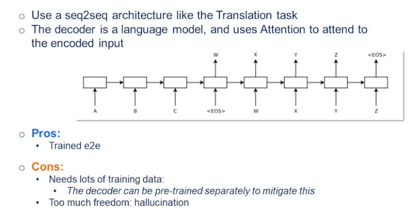
Now we want to be talking about the neural models for this task. We’ve skipped all the traditional models for summarization that existed before neural models were the norm.

The starting point for the new wave of summarization systems that use a neural network was started in 2015 by the paper linked above.

They used a seek-to-seek model that was introduced just a year before, which would take an input and would generate a target output token. The underlying architecture was an RNN. So this is your encoder and you get the end-of-sentence signal that it has ended. And then basically you would get the output of the encoder and initialize your decoder and you generate the outputs word by word. So you generate X and you give X again to your model and generate Y, etc etc, until you hit the end of sentence. And this is where you end the generation.

this is really similar to the translation tasks and the architecture that was used for that. The decoder is basically just a language model. You can imagine that this decoder not only looks at the previous token but can actually attend to all the steps of the encoder as well. And the underlying architecture at the time was RNN. But you can imagine you could have a seek-to-seek model from transformer models that would do the same thing. And this is what we would talk about more.

This makes abstractive summarization much simpler. In terms of formulation you don’t need a pipeline that traditionally you needed a surface realization and things like that planning. So usually it was a pipeline you plan and then you surface those words. So here everything is trained end-to-end. So can you just give the original document as input you encode it and you decode the summary. And again similar to all other seq2seq models it uses teacher enforcing.

one problem for this technique was that it needed a lot of training data because everything was trained from scratch. And the model needed to learn a good language model as well. Faithfulness aside and things like that it needed to be a good language model to spit out good English or good language. And that’s why there’re variations of this that separately pre-train the decoder so that you start with a pretty good language model to begin with so you don’t have to teach all the grammar and everything. Again on top of it you can pre-train the encoder on other tasks and then just use on this one.

So there are a lot of improvements that you can put on top of this simple seq2seq model to make it better and better. And this is something that has been done for RNN as well.

But a huge problem with this was that it had too much freedom. And especially this was not a model with a high capacity so you couldn’t really pre-train it that much. So in terms of choice of wards and everything it had too much freedom and it would hallucinate a lot. And that was a huge obstacle toward its deployment in real life.

Pointer-Generator Networks

What made a huge impact and made this model much more tractable was a paper from Stanford that introduced the copying mechanism.

Get To The Point: Summarization with Pointer-Generator Networks

Think of the copying mechanism as a middle ground between the faithfulness of extractive summarization and the versatility of abstractive summarization. Here the model decides whether it has to copy from the stores, extractive behavior, or generate from its own vocab, which is abstractive behavior. Furthermore it has to learn at each step which one it wants, and which method.

here I brought this example from the original paper. And I encourage you all to read this paper on your own.

And so imagine you have the source text here and you are encoding it. Again the underlying architecture was an RNN here but everything could be done with transformers as well. And once you’re encoded this so you start decoding the summary. And at each step in the summary you’re looking at two different distributions the green one and the blue one.

The blue one is a simple attention mechanism that at the time was introduced for translation. You want to know which of these words I have to attend more. And that’s why it gives a distribution here. And so for the next word for example here after Germany then it was produced. Then Germany then you either want to be talking about victorious or when probably it gives the highest probabilities.

The other side of the spectrum, the other method, that they could generate is through its own vocabulary. So it has its own vocabulary whatever that number is. Usually for such a task you would use probably tens of thousands of words or subwords. And you have a distribution over those as well. So here the one with the highest probability is very similar to when like beat.

Now that you have these two distributions you have to decide which one of those you’ll want to use. And here similar to all the neural network architectures you don’t have a discrete decision. You always have a soft probability. So you have this distribution and you have the attention distribution. And you combine them with a probability in a soft way and then you get the maximum probability and reward that it corresponds to.

you can imagine that if the probability of a copying was 0.5 so it means that you basically just combine these two distributions together. So for each word you average out the probability that it had in the attention mechanism as well as in their vocabulary and distribution. But usually that probability is much sharper. So as I said it’s never one or zeros never either or. But a lot of times it could be like .999 or something like that. So you’re pretty sure that you want to copy here.

Through this mechanism you have the flexibility to choose if you want to copy something or generate it. And this was a huge step towards more faithful abstractive summaries in the neural networks that the model now its degree of freedom was brought down a lot. So it could just easily copy and didn’t have to make everything up itself. There are more details in this paper. So for example you want to make sure that it just doesn’t always copy. So there are different losses that could be added to it. But this copying mechanism is something that was used after this task for a lot of different tasks as well. That when you wanted this explicit summaries explicit copying to happen.

BertSum

In the last part of the lecture so I want to talk about the pre-trained models for the summarization task which have set the state of the art for the last few years.

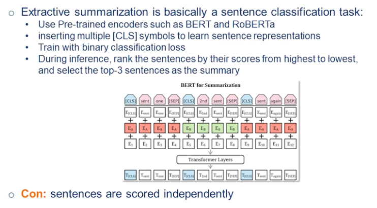
The first of these is BertSum

BertSum as could be inferred from its name was using BERT model pre-trained encoder to do the extractive summarization. So extractive summarization can be thought of as a sentence classification task. If you confine yourself to only use full sentences which would guarantee that you’re going to be grammatical and you’re going to be probably cohesive enough this is something that exactly would be a sentence classification and you don’t have to worry about sub-sentences and sub phrases things like that.

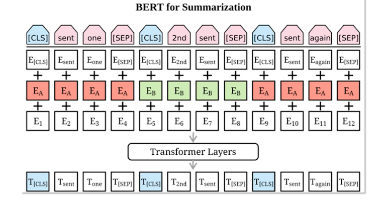
let’s go over the example here and see that how it was done.

Imagine you have a bunch of sentences, where for each sentence we add an CLS symbol before it. So this is something that’s in the original BERT Architecture as you might know that the CLSO class token was added at the beginning for the classification tasks. So here we have this. For each sentence we have to make a decision that we want to include it in this summary or not. So that’s why that we have one class label for each sentence.

Next we add the word embedding and then this is the segment embedding and then a position embedding and the common stuff and the transformer and we give it to BERT.

Once you decode it, your target is that you want to predict the class label for each of the sentences. So one thing to add is the separation token that you pull it before each sentence. I don’t think it really matters here honestly because you have the class label so the model knows that when the sentence is over when you see a new class label but they just decided to have this separate step token here as well. Usually when you have multiple input that you want to give to the model and you want to make sure that it understands that these are two different sources, or two different things to be treated differently, then you add a separate token. But here they had at its class as well as the set but at the end of the day you want to predict this class labels.

For the loss we use just a binary loss that each one is either zero or one. Then so during your training for each sentence you’re doing that loss and then during the inference so each class label as predicted is going to be a probability between zero and one. Then they are ranked from highest to lowest and depending on the summary length that there’ll be once they take the top K sentences. In the original paper I think they were doing top three sentences. So that could be another hyperparameter in your model depending on the dataset that how many sentences you want to pick.

This performed pretty well. It’d be the state of the art for I think CNN & Daily Mail datasets but obviously it doesn’t work for abstractive summarization. But one thing even the event about extractive summarization is that it was scoring the sentences independently. So even though the BERT model is contextualizing everything as long as it’s in its attention span. So all these scores they have been contextualized. But the BERT model is not going to be trying to make your model as least redundant as possible and there could be two sentences that they mean similar thing and both of them are important sentences and the model could score both of them pretty high. Even though in a good summary you either pick this one or that one not both. And this is something that has been studied after this paper as well that you don’t want that once you have this course the only thing that you can do is to basically just pick the highest one and those scores and you’re not considering that what you have picked before.

So there are methods on top of this that in order to make a decision not only looks at this score but it looks at what you have already picked. So for example when you pick the highest scored one then that probably is the most important center you want to pick anyway. So once you pick that then the next ones the score for them is going to be relative and it’s going to matter that which BERT centers you picked. This way redundancy can be brought lower. But again in its original form it worked pretty well and it has some follow-up papers like match some that you guys can look on your own. I strongly recommend doing that.

Abstractive Summarization: Pre-Trained Models

This section we look at a new class of models that were first intorduced in 2019/2020. At their core these were just pre-trained seq2seq models like such as BART and T5.

these generative pre-trained models fall into two classes.

The GPT class: that are decoder language models
- this means that there is no encoder
- it’s just one decoder and everything is trained token by token.
the auto-encoders, On the other hand are truly a language model
- here you have a corrupted original sentence and you predict the correct one
- this class includes BART and T5.

All these models are really good pre-trained models for generation that you can fine tune for different tasks such as summarization. Because these models are pre-trained very well, they don’t make many grammatical errors unlike those earlier LSTM models. Everything is pretty coherent. Although it could be nonsensical, or unfaithful, but usually coherence and grammatically is not a problem for them.

So in order to finetune for this task. So it was GPT2, that introduced the prompting method and then it was followed up and the next versions of GPT as well. So usually the way that it work is that you give the original document to it and then you add TLDR at the end. Or you could give it in summary colon and then you prompt it to predict a summary word by word for it depending on the context that it has consumed.

So good thing about this is that you can do this without any training. So it’s all zero shot. You can get the decent summaries. It’s not comparable with supervised techniques at least for GPT and stuff. Right now with the advent of all the models like ChatGPT the quality of the zero-shot summaries that you get are extremely good. But still if you have a supervised data there are going to be in terms of performance dwarf compared with them.

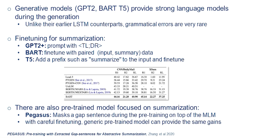
Then next class of models that you need to finetune is that of BART and T5. In BART you just finetune with the paired dataset like you give the input and you give the output and that here is the summary and you find Jean Piaget model. In T is usually better to add the prefix as well. But it could work and learn without that as well. Once you do that you fine tune it and you can get the abstract of summaries with this.

Here we can see the results table from the original BART paper and it has a list of some of this methods. There was a huge gap in terms of performance with previous methods.

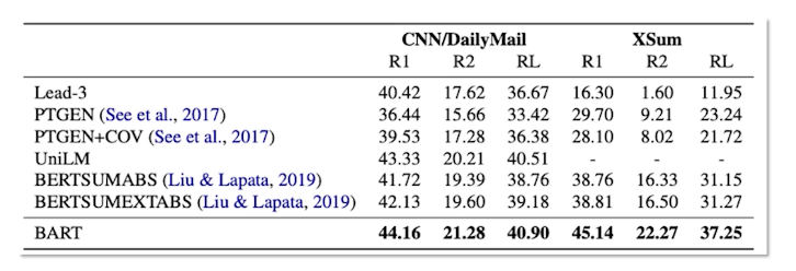
For something like CNN/DailyMail one rouge score is huge like consistent improvement. Here you can see that especially with the for the XSUM summarization which is extreme summarization. Their performance is a huge gap with other techniques and this is where these models really shine. For something like extractive as you can see Lead-3 is a previous summary for CNN/DailyMail is that R1 is just over 40, which is non-trivial at all. So even something that we discussed the point or generator model with the copying. It dwarfs state Lead-3 which is a huge baseline.

But this model BART is versatile enough that could give both the extractive summaries as well as abstractive depending on what supervision it’s gotten. There has been a lot of summarization focus pre-training as well. Maybe the most notable is Pegasus that it on top of token masking like BART it would do sentence masking as well. And it showed that it had some improvement on top of BART. But it’s been shown that a lot of times if you carefully finetune these models, the pre-trained models for this task, you usually don’t need specific pre-training for different tasks. A generic pre-trained model can provide pretty much the same gains.

Hallucination in Summarization

Finally I want to discuss a little bit more of the hallucination problem. And now that we have this pre-trained language models that as I mentioned the coherence naturalness and grammatically are not issues with this model. But it’s still deploying a model like BART in real life setting is pretty challenging for a task for summarization. And the biggest problem is the hallucination and the possibility of it. Because you don’t want to be making things up that never existed and make a PR issues and things like that.

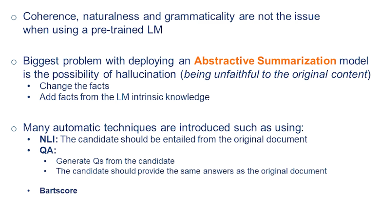
So in this models they’re usually two types of hallucinations that could happen. One is that you change the facts from the original document that for example someone was born in some year and you generate some other date or you add knowledge and you add facts. those facts could be wrong or they could be correct. This is something that comes from the language model intrinsic knowledge. And these models have huge capacity to memorize the Internet knowledge that they have been pre-trained on. And that’s why they sometimes they can just spit out something without looking at the document to see if it exists or not.

just for this task this hallucination there are a lot of different techniques and metrics that has been introduced for models like Bart but in general it works for any methods. But this is something that is much more recent metrics. So we did discuss the BARTscore and how it calculates the hallucination.

But I want to mention two other techniques as well.

One is the natural language inference which is a entailment task. Entailment task are two sentences could have three different relationships toward each other. One can either entail the other one or it can negate it or it can be neutral. Here we have the summary and we have the original document. And we want to be in a way that original document entails the prediction that we have. Which means that all the facts to it have been presented in the original documents as well. So there are a lot of inference datasets and that’s why was one of the good things about this method. But one of the problems with this is that language inference is a really hard task. And different datasets they’re not really even generalizable to each other it really depends on your domain. So it’s not a problem that has been solved. And then we said okay now when you solve this we go and use it to other metrics. So that’s why that there are some push back against this metric as hallucination because itself is a really hard task as it has shown mixed results.
The other thing that could be more promising is using question-answering for this task. So question and answer and you might be familiar that you have a document or Excel document and you have a question and you want to answer it. Dual problem for this is question generation. That you generate a question from the document and then you try to answer it. So the way it works as a metric we generate a lot of question candidates. These dispersions are generated from the candidate summary. And now those questions they have to have the same answer in the candidate summary as well as the original document. So if you generate enough questions and you can calculate the probability that this is faithful or the reference and the candidate summary was faithful or not. So usually I think there could be like questions depending on the left but questions questions that you will compare the answers from the original document and from the reference. And if they match like nine out 10 of you get a score like % or if there’s like a it’s % faithful.

This is an active area of research and this is something that again still there’s a gap between human evaluation and the automatic metrics. And if you’re interested you can study more and you can read more papers on this and see the newest techniques.

Module 10: Machine Reading

Machine Reading

Machine Reading: Extract factual knowledge from unstructured text web and palcing it into a structured knowledge base.

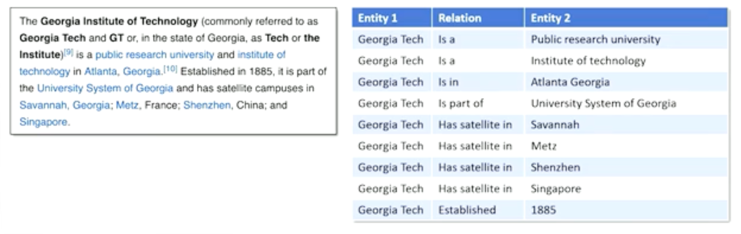
The main idea is about information extraction, open and closed.

closed information extraction - a fixed set of types of relations:
- Example: established, is a, has satellite, provost, etc
Hand-authored rules
- Example: Look for a sentence with the word “established” and a date
Problems:
- New year of expression information
- new relations can emerged
- Too many relations to anticipate
Open information extraction - Extract structured knowledge from unstructured text without knowing what the entities or relations are in advance
- No prior knowledge on what the relationships are
Unsupervised acquisition task

Why must we do this in an unsupervised way?

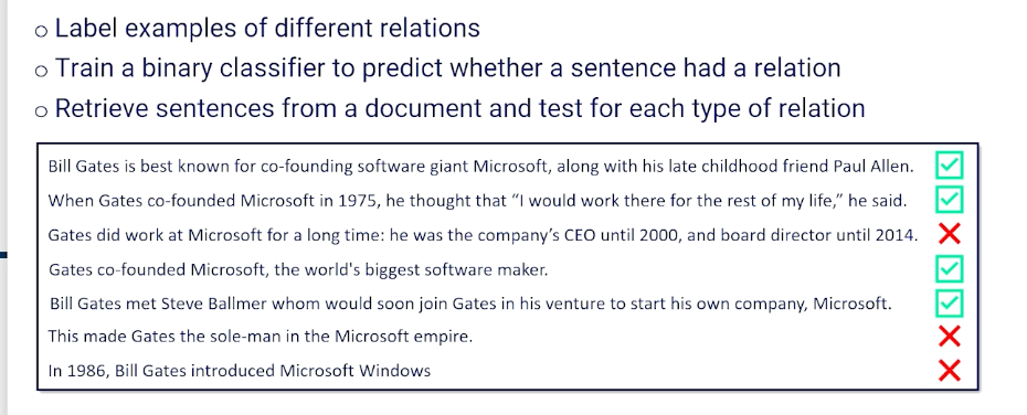
It is not impossible, but difficult. We need to go get a corpus and we have to label examples of different relationships. Once you have this dataset, train a binary classifier to predict which sentences had this particular relationship in it, and use it to go through any sentences I want and test the sentence to see if it has that particular relation that we are looking for. And this has to work for many types of relationships which is not a good idea.

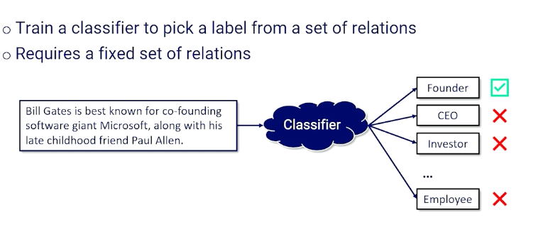
Things gets even more complicated - what if we have multiple types of relationships? Then we need to consider it from a multinomial perspective.

Distant Supervision

Instead of manually labeling, automatically derive labels from an existing knowledge base.
Assume every entity that is related to another entity in a sentence is a pstive example
- “Jack loved his sister Jill very much”
Assume every entity that is unrelated to another entity is a sentence is a negative example
- “Jack and Jill went up the hill”
But how do you know whether two entities are related in a sentence?

We call this distant because we haven’t gone through and directly built out the labels for the dataset, but we’ve written a piece of code or a process that can guess what those labels are. Those labels might be wrong in our ultimate dataset. So we’re not directly supervising. There’s this layer of indirection between the supervision that we want to provide to our algorithm and what the data actually has.

Now as humans can look at these examples and we can see those relationships and we configure these entities are related these aren’t. But algorithmically how do we know whether two entities are related in a sentence? And this is the problem that we’re going to turn ourselves to.

Open information extraction requires learning a way to recognize relations without labeling
- Do this by using the Syntax of sentences provide strong clues about relations

Part of Speech Parsing

We have to talk about POS parsing to dive deeper into machine reading.

Syntax: The arrangement of words and phrases to create well-formed sentences in a language

Humans can understand even if its not well formed
But better for machines if they are
Semantics arise from Syntax
- is the meaning of words and the meaning of sentences

Example: “Jane Loves science”

3 words, with a very simple syntax but the semantics are quite complicated
- Jane: is an entity, person. T
- science: is a concept
- love: denotes a positive relation/affinity
We know that Jane has positive feelings about this idea of science these words have a whole bunch more behind them that we want to be able to get from these words.

That’s what we mean when we talk about semantics arising from syntax.

Different kinds of words take on different roles and have different rules that apply to them in a sentence based on where they’re used in a sentence, and what we want that sentence to mean.

Here’s another example that’s actually a little bit ambiguous but is syntactically well-formed, syntactically correct.

Jane wrote a book on the moon
- did Jane write a book about the moon?
- did Jane write a book while living on the moon?
- you actually cannot tell just by looking at the sentence which of these two meanings we should extract
Ex2: Her drive was torn up
- which is the verb: drive or torn?
- drive could be the act of driving or it could also mean the noun driveway
- torn could mean “ripped apart” or it could also mean falling apart
- So is a driveway torn up or is her car like the thing that she is driving falling apart?

As you can see here the correct way of us determining what words have what roles in a sentence is actually a hard and non-solved problem

Parts of speech - a category to which a word is assigned in accordance with its syntactic functions

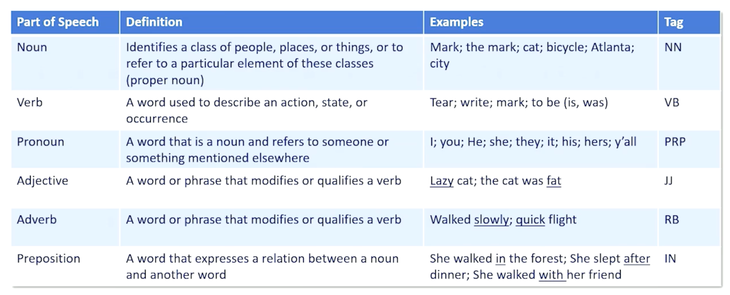
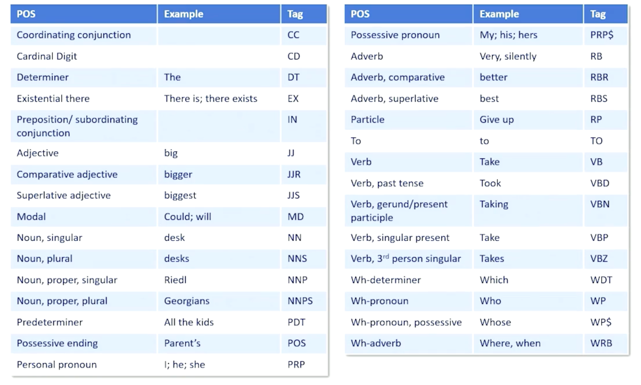
So, how do we do parts of speech tagging - which is associating these different roles to the different words in a sentence?

Assign a part of speech tag to each word in a Sentence
Probabilistic approach: Set up a dynamic bayesian network

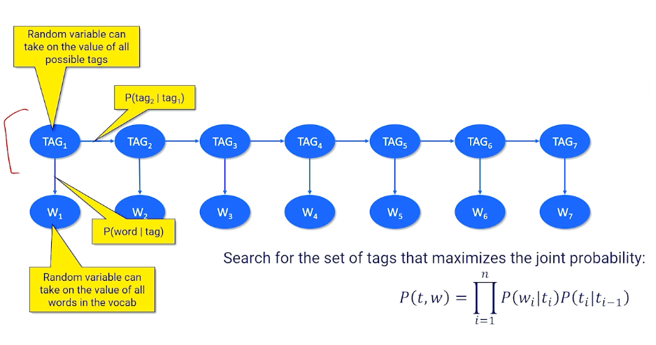
To give an example:

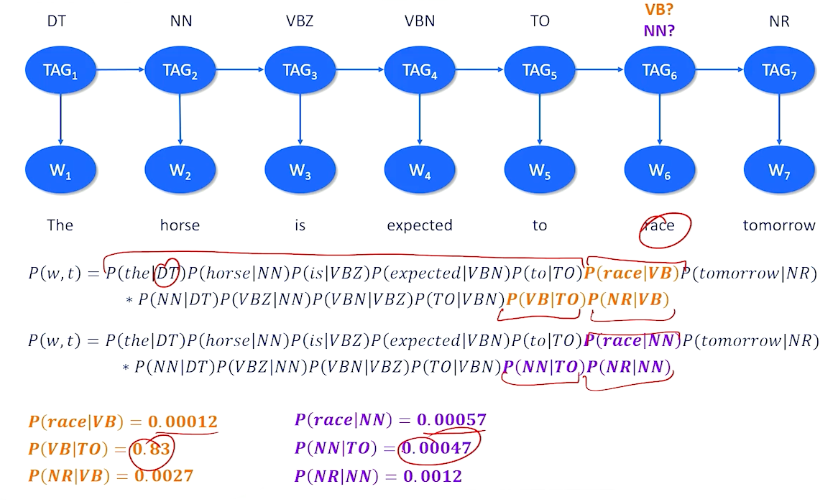
We might have a particular document like the horse is expected to race tomorrow and we might take a guess that there are particular tags that should be assigned to each of these words. And in most cases and this is one well actually two possible mappings here. And in most cases there’s a really strong correspondence between the tags probablistically in words like “the” is a determinant, horse is definitely a noun, “is unexpected” are two parts of a verb phrase or two is a special type of part of speech that is setting up something. The one big question here is race. Race is a word that can be a verb but it can also be a noun. Should I choose verb or should I choose noun which is the right choice here. To do this we can turn to the statistics we can turn to the probability. We can set up a giant joint probability equation where we look at the words and all their tags.

If I pick the right dub tag for the then I should have a high probability here. The question is do I have a high probability that race is a verb or not? Do we tend to see the word race when I know that there should be a verb here? And we also want to know what is the probability that I see a verb following a two and a relative noun following a verb. And this might be different. So this other possible mapping would say race is a noun was the probability I see the word race when I am expecting a noun do I tend to see a noun following a two and so on and so forth. And we can basically decide whether we want race to be a verb or a noun tag by looking at the different probability of the entire sentence. So everything is the same except these two parts but what we can see here is race is not a very common verb not also a very common noun. But we tend to have a very high probability of seeing a verb after a two and we don’t tend to see a high probability of a noun after a two. So if I had to multiply everything up together again we’re basically say this is the most probable explanation. This is the most probable tag that we'd want to use or most probable set of tags we’d want to use for this sentence. Now how do we make that determination? So I gave you the tags and then we chose between two possible tags in one spot.

How do I figure out what all the tags are. We all have the word we don’t have the tags. We need to do something called the most likely explanation which is basically a search for the sequence of latent values these tags that would most likely admit the observed words.

Now we can do this the brute force way. We can look at all possible combinations of tags for all possible positions and then we can compute the probabilities like we just did. That would work but there’ll be very computationally expensive and exhaustive. We don’t necessarily want to do. But there’s one little trick that we can use to speed up and make this more efficient. We can use something called dynamic programming. And what we’re going to do I’m not going to go into how dynamic programming works but it’s built on the assumption that for any one choice that we have to make in this entire sequence that the most likely choice for that one time slice means if we can make the best choice there that means we will ultimately find the best overall choice. So it the best overall explanation is built of a bunch of local optimal choices along the way. So all we ever really have to do is make the best choice at every single time slice and we’ll end up with the best part of speech tag at the end. This isn’t guaranteed to work but it’s a pretty strong assumption here and it tends to work. So if you’re interested in this you can consult some background knowledge on how to set up a dynamic programming algorithm and what the right algorithms are that actually can solve this problem. But now we need to take this knowledge about parsing in parts of speech and bring it back with us and return to the issue of machine reading.

Dependency Parsing

Dependency parsing is a theory that basically says that we can build graph structured syntactic analysis of sentences that will help us find these relationships. Dependency parsing is a linguistic analysis technique used in natural language processing to uncover grammatical relationships between words in a sentence.

Words have relationships to each other
Graph-structured syntactic analysis of sentences
Root of tree is the verb
Arcs are dependencies with types

So to give you overview of this means:

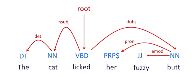
For example we might look at this lick verb and we might decide that this is the route so that this sentence is about the lick action. We might notice that the cat is the subject the licker and the thing that is being licked is the butt which is the object. So we have subject-verb-object. Then we have other information like fuzzy and butt is modifying fuzzy and her modifying information about what we know about butt and cat tells us which cat and things like that. So the idea is that we should be able to build this graph relationship between all of these words and that’s will provide additional information that we need to ultimately do our knowledge extraction.

The most successful way of doing dependency parsing is something called the shift reduce technique. The idea here is the bottom-up technique to build a dependency graph that really explains how different words are related to each other and gives us both the relationships and the types of relationships.

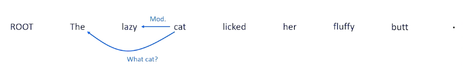
Let’s think about the sentence at the left. We can look at different combinations of words and tell us whether they’re related to each other. So we’re not sure about “the lazy” but we can look at cat and these might be related because the tells us which cat we’re talking about, it’s the cat. Likewise the word lazy and cat seem to go together because the word lazy is modifying the cat, it tells us something about the cat, it’s an adjective modifying the cat. We can also look at the relationship between cat and licked that this is probably telling us that the cat, the entity, that is doing the licking, doing the verb.

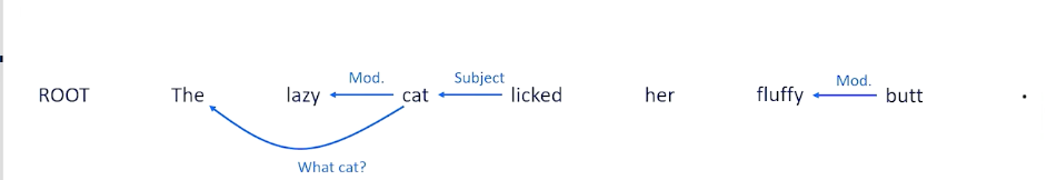
We can also look near the end and see that fluffy is a modifier. It’s an adjective that’s probably modifying the word butt that seems to be the most likely thing that is modifying. And this is telling us something not about fluffy but it’s telling us something about the word butt is talking about, who’s butt, We’re talking about what is being licked. Was it her was it butt. Well the probably the right parse here is that the object the thing that is being licked is the butt. And the punctuation tells us that the event is done.

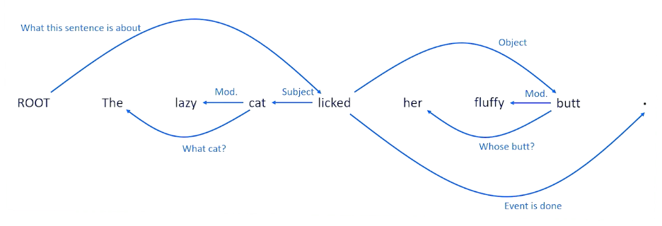
And the ROOT is going to tell us that this is what the sentence is all about. So the sentence is all about this lick action and which terminates once we know everything about the lick action and the entities involved in the lick action.

Shift reducing Parsing

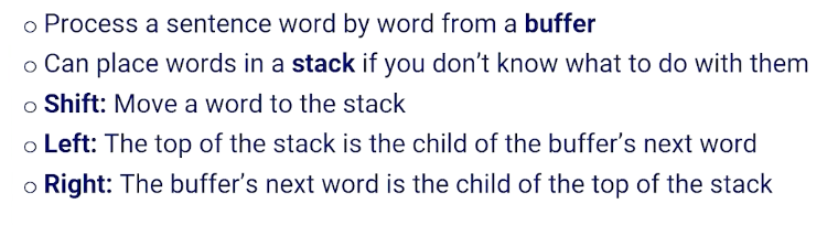
So shift reducing has two key data structures that we’re going to use. The one is called a buffer and this is just the order that the words are presented to us in the sentence. So this is going to allow us to process and walk through the sentence word by word. We store the word in a buffer. We also have something called a stack which is basically an extra data structure off to the side which basically says if you don’t know what to do with any word in the buffer will just push it onto the stack and hope we can figure out what to do with it later on. Now there are three operations that we care about.

The first operation is called the shift which basically means take something from the buffer
- first word the buffer push it to the top of the stack.
- Basically save this for later because we don’t know what to do with it.
The left operation basically means we have found a relationship and this relationship is from the top of the stack a word that we had pushed off to later is somehow related to the next word in the buffer.
the right operator which basically says the next word in the buffer is related to the top of the stack. So in particular the buffer is the child or the top of the stack whereas left means the top of the stack is the child interdependency of the buffer.

Let’s see this play out in an example

Dependency Parsing: Example

Here is the same example again, the lazy cat licked her fluffy butt.

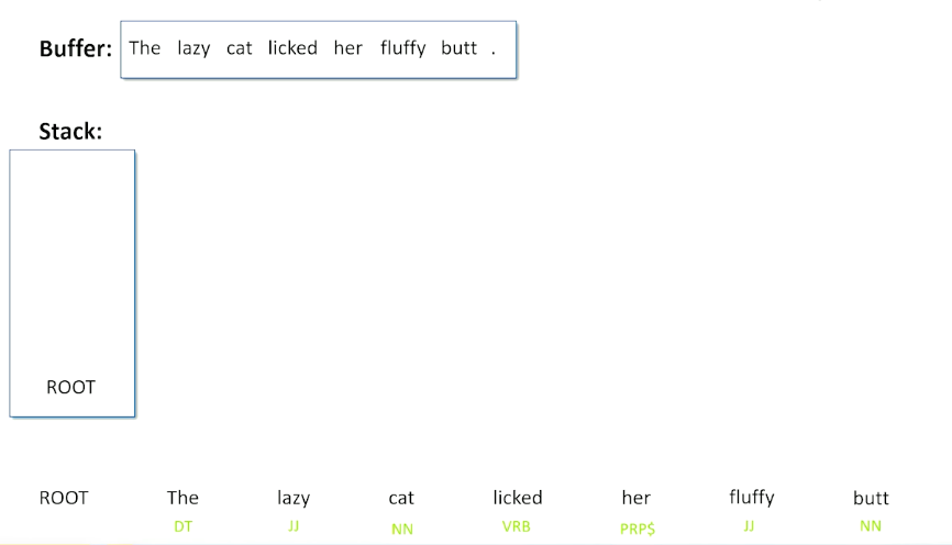
we can see that the sentence is in the buffer ready to be processed and we have the stack. One special thing I’m going to notice I have added this special term token root, and that we’ve pushed the root onto the stack. We start with the root on the stack. We know we are done with the entire process dependency parse when the root is no longer on the stack, meaning we have finished everything off and there is nothing to think about anymore.

At the top right corner, We will look at the different relation, the operations we do. So as we try to parse this, these will be the operations shift left or right that we attempt. To kick things off, if there is nothing on the stack except for the root, we don’t really have anything to do because although relationships are be there between the stack and the buffer or back from the buffer back to the stack. So if we do not have anything but the root on the stack, then the really only thing we can do is shift, which basically means take the next word in the buffer and push it onto the stack, no relationship is being to created. So we are going to shift the word the into the stack:

Now, there is something on the stack and still have our buffer. But when I look at the word the and lazy, it is not entirely clear to me that those two things to together. So i am going to grab the lazy and I am going to shift it onto the stack as well. Maybe I will be able to do something with this a little later.

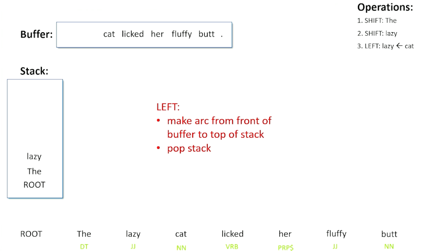
So now the next word in the sequence is the word cat and now this time we have a choice to make and it seems like a reasonable choice to make is to do the left operation, which is going to create a relationship from cat from the beginning of the buffer to the top of the stack.

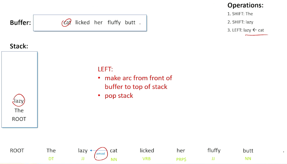
In this case, the relationship is an adjective modification, so lazy is an adjective and we see an adjective preceding a noun, we could probably make a reasonable guess that this adjective is modifying that noun. So we have this relationship between lazy and cat that we can go with. And when we do a left, we both create that arc, and we are also going to pop that stack - we have figured out what lazy is all about, we are done with that and off it goes.

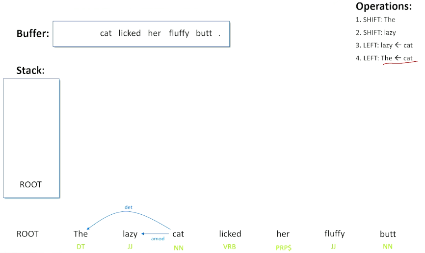
The next thing we can do is we can now look at the cat and the word the. In this case, when we have a determinant the, and a noun together, it is probably a reasonable guess that the is telling us which cat determinant of the noun. Once again, we can do a left shift, basically which will create the relationship that cat and the go together, and remove it from the stack.

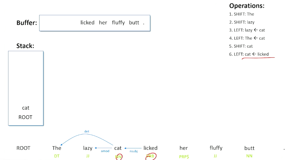
Now, there is nothing on the stack except for the root, so will shift the cat onto to the stack. So if we can deal with that a little bit later. That allows us to onto the word licked. And here we can look at cat and licked, and there is a nice thing happening here. When we have a noun and a verb, the noun is probably the subject of that verb, so we will go ahead and will do a left operation, and create the subject relationship, saying the cat is the subject of the verb and we are done with the cat.

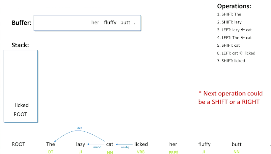
Now, it is an empty stack again, we pushed lick into that, we are going to do a shift. We are about to see the word her, and it is really not clear what to do here. When we are talking about licking and her, the top of the stack and the front of the buffer, it is entirely plausible that the cat could have licked her versus the cat could have licked something else. When we see a verb and a pronoun, that is one possible thing that can happen.

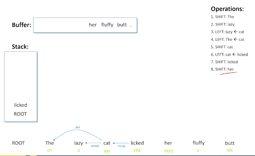
So we are going to have to make a decision here, the right decision is going to be to do a shift. The reason why we are going to do a shift is because if we did not do this, we end up with some extra words that we did not know what to do with that would not fit into any other relationships. Now we do not know this at this time, let’s suppose the algorithm has to make a guess here and let’s just suppose it makes the guess teh right thing to do with is shift.

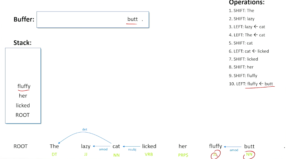
Now, we have fluffy, and her, her fluffy - we do not really know what to do with pronouns and adjectives following pronouns, so we are going to do another shift, and shift fluffy onto the stack. Now we have the relationship between top of our stack and buffer. So we have an adjective preceding a noun. Once again, we probably think there is a pretty good guess that the word fluffy is modifying that noun, so go ahead and do a left operation here make the relationship and say fluffy is modifying the word butt.

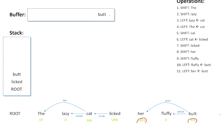
Now we see a possessive pronoun and a noun together, looking at the top of the stack and the buffer, and we can make the guess here that probably her is saying something about who owns the possession of the butt. So the pronoun is related to that word there, so we do a left operation and now we have understood what butt is all about. We are done with the pronoun there.

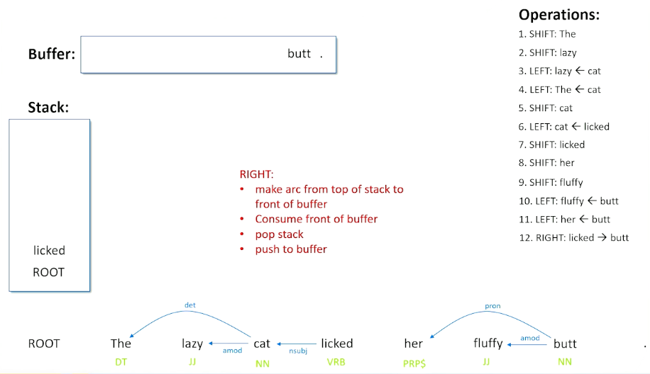
We still have butt to deal with and now we have something here that we have not seen before - we have the possibility of making a right shift. The right shift basically says that there might be a relationship going the other way from the top of the stack to the front of the buffer - because we see a verb and we see a noun (licked and butt) and a noun is after the verb, so that is probably going to be the direct object of the verb.

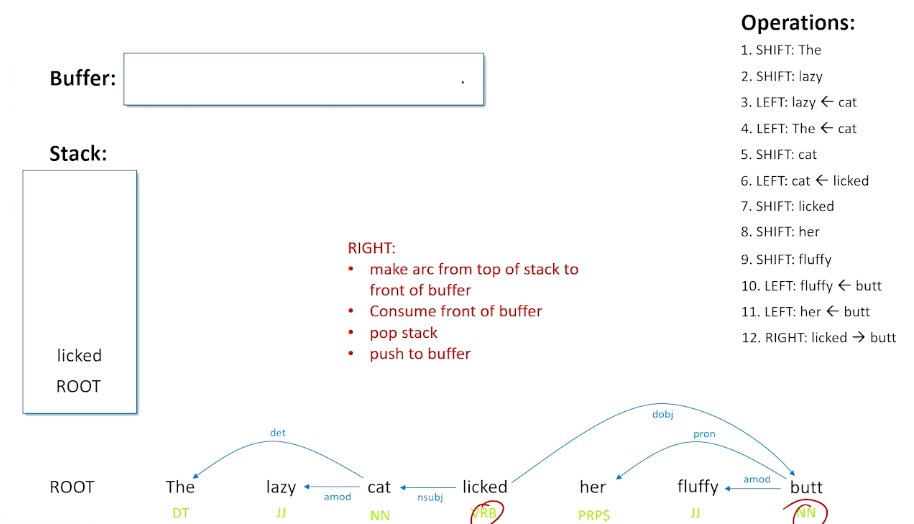
Now rights are a little bit more complicated, what we are going to do is consume the front of the buffer and we are done with butt and there is a relationship that we just made.

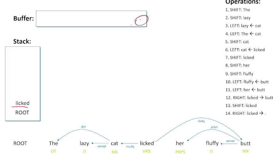
But we also take what was top of the stack and put it back on the buffer saying we might not actually be done with this word licked. There might be other things we have to consider about this as well as when we do a right shift. Now we are back in a situation where we have words on our buffer, but nothing on our stack, so we are going to actually shift licked back to the stack (did not have to happen that way) and we are left with a punctuation. So when we have a verb followed by a punctuation, we can do a right and we can basically say that that this is the termination of what the sentence is about the sentence is about the verb. So we put the punctuation relationship in here and because it is a right shift, we kick the punctuation out, and once again return lick to our buffer to make sure we are not done with the word licked.

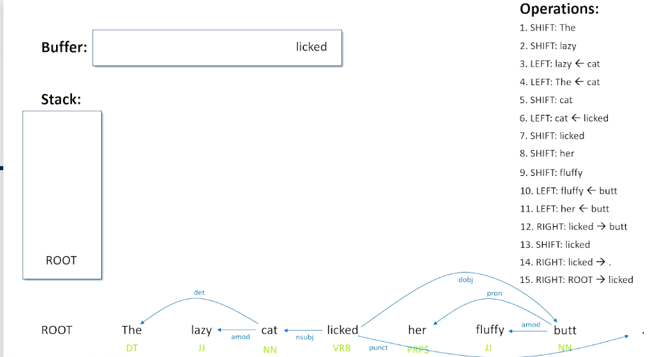
One last right shift, to do and this is a special rule that basically says when you have the root and a verb or the root and the last word and sentence, then whatever remains in the buffer must have been what the sentence is actually about.

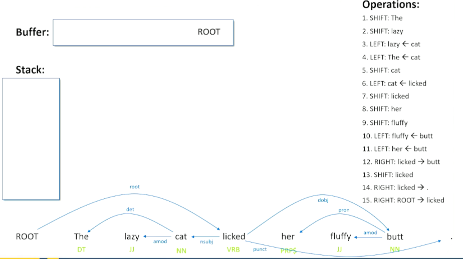
So we do a right shift from the root to licked, so we say licked is the root, we kick that off, root now becomes part of our buffer and this is our terminal condition. The word root has moved from our stack to our buffer, that means we are done and have addressed every single word in the sentence we have found its dependency to every other word.

Learning

Seems to be doing a lot of hand-waving along the way, in particular when we had to figure out what was the direct object of the verb licked, was it her or was it butt and basically did a hand-waving and said well, let’s wait on the word her because we might see something better but how did I actually know that?

How do you know whether to shift left, or right?
We can actually learn a classifier
- Given a stack, a buffer, parts of speech tags,
- Output shift, left, or right (and dependency type)
But how do we build this dataset?
- Distant supervision
- Annotate a lot of sentences with Dependency graphs
- Run stack-reduce, backtracking when necessary to find the known graph
- X: partial parses of sentences (buffer, stack, POS tags)
- Y: Best shift-reduce action (shift, left, right)

Basically this tells us these are the sets of shifts lefts and rights we have to do to get to the stack reduced to match the actual answer according to humans what the right parse is. What that means is then if we look at that process of shifting, lefting, and righting what we end up with is a bunch of partial parses of sentences. So basically the shift reduce at different stages in processing a sentence. Which tells us at any given moment what’s on our stack what’s in our buffer and what the parts of speech are which is exactly the information we want that our input to our classifier. This also tells us which was the shift left or right that we had to do to make the correct annotation work according to our human annotators which tells us what our Ys should be. So we can infact generate automatically through repeated uses of stack reduce backtracking and trying different options until it gets it right to automatically produce a dataset that we can then train a classifier on it. And then once we’ve done that we can use the classifier in any future stack reducing that we need to do to create dependency parses.

Open Information Extraction

Recall that we are trying to take unstructured text to structured knowledge such as (subject, relation, object) triples. So for two entities in a sentence, a subject and an object, they must be related when possible, how they are related by a particular relationship.

To give you an example of this, consider OBama was president of the United States from 2009 to 2016.

Open information extraction should be able to tell us these following structured triples exist:

< Obama, was, president>
< Obama, was president of, United States>
< Obama, was, president of United States from 2009 to 2016>
- There are different ways of looking at that sentence and figuring out what the entity is. So president is one entity, but also president of the United States is also another way of expressing an entity.
- Name entity recognition is a little hard and when in doubt, you just look at all combinations of ways of talking about an entity and worry about things later on.
< Obama, was president from, 2009 to 2016 >

So how do we come up with these particular triples from this particular sentence, and dependency parsing is going to be the key intuition we have here:

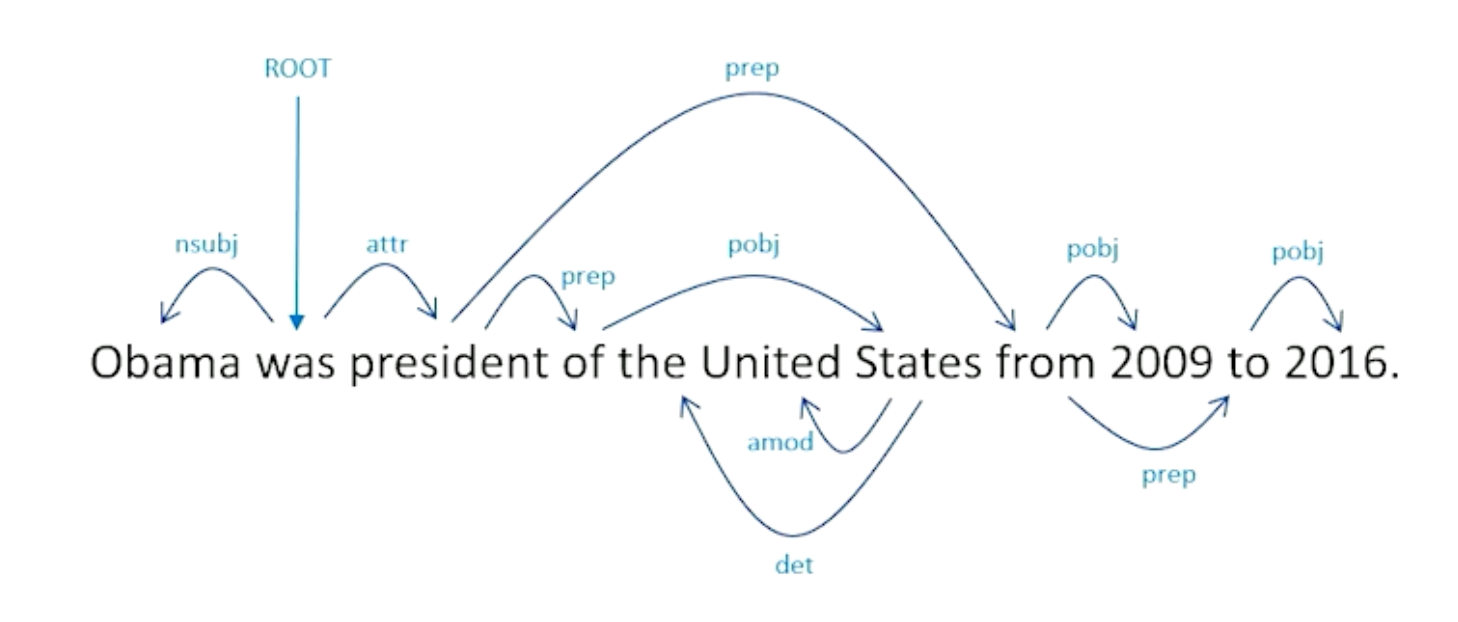
This tells us how every single word is related to every other word. Our named entity recognizer came up with a complex noun phrases. Obama was easy, but things like president of United States involves not a single word but multiple words. Same with relationships here, relations can involve multiple words instead of single words as well. How exactly did these tuples came about? It turns out to be a straight forward process.

First thing we have to do is figure out what all the entities (Obama, president) are, list all those out, and then just figure out how we get from one entity to another. So we are literally going to find these entities inside our sentence, and going to trace through dependency parse to get from one entity to the other.

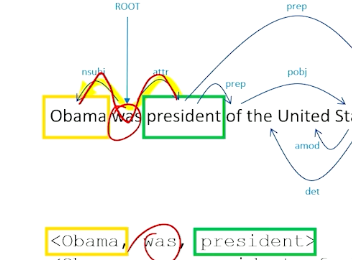
So to get from president back to Obama, we can follow the yellow path, which basically take us through was the attribute to the subject of was being Obama. So if we walk this particular path of the graph, we go through the was word and was becomes our relation. So now we know how obama and president is related.

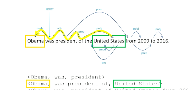
We do this for all ways of expressing all entities in the sentence. We look for OBama and the United States, how are they related to each other, while we walk through the object back to the preposition, so we walk through of president was back to Obama, so was president of becomes our relationship there.

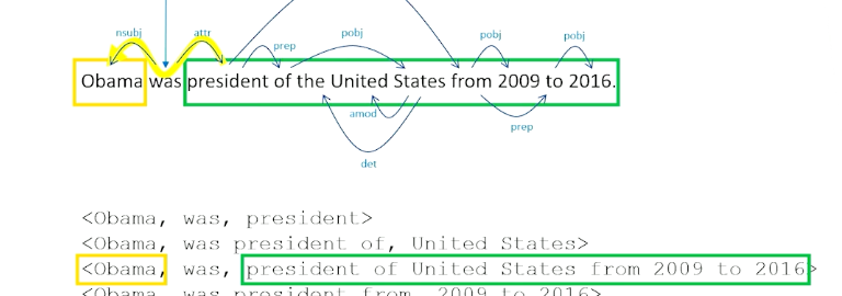
President of the United States 2019 to 2016 is also a way of expressing an entity, so we find that, we find Obama, we again can walk through the word was by following the arcs in our dependency parse. So we get was for the relationship here.

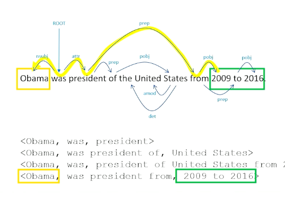
And 2019 to 2016 is also an entity, So we have to walk the graph here again. This one is a little interesting, we walk through the word from, that takes us to president and was, so was president from, we can actually skip some of these intermediate words to figure out that this is the core relationship between Obama in 2019 does not really involved the words United States.

Now, the useful thing in terms of this now is once we have collected all these up and put them into a knowledge base, is they can tell us all the different ways that different entities are related to each other. And this can involve and is primarily used for question answering. So what do these triples tell us? - They tell us things about who Obama was.

He was a president
What was he a president of?
- The United States
When was he a president?
- 2019-2016
All these things can be answered now by simply trying to match parts of a question to what is known from the documents.

One of the predominant uses of open information extraction is in fact to do question answering about documents. We want to be able to use these structured pieces of information that we pulled from these unstructured text to be able to answer questions about those texts, as well as about the world that the text describe in general.

For example Obama was the president of ? . We should be able to figure out the word clearly should be United States. That is very nice when the question match very closely to the structure triples that we are able to extract. And we should expect to see that because theoretically it is easier to work with structured knowledge than unstructured knowledge.

And when we do not have perfect matches, we can still fall back on the distributional approaches, so we can look at the cosine similarity between different parts of a sentence and then different pieces of information we have in our structure tuples. So in the case of the example when was Obama president, we do not have an exact match from our triples but we can see that this question is about the entity Obama, was president from might have a very similar cosine similarity to when was and one was president. We might be able to figure out that when was president is a very close match or cosine similarity enough to the relationship was president. In which case all we have to do then is figure out this is figure out that this is probably the best triple that we have in our entire knowledge base. And then we can go in and find that one particular piece from the triple that the original question didn’t actually have. And in this way we’re able to make reasonably good guesses about the answers to different questions even when they’re structured a little bit differently from the knowledge we have in our knowledge base.

Now there are pure neural approaches to machine reading and to open information extraction. Historically they’ve not been as robust in creating structured knowledge from unstructured knowledge as the techniques the unsupervised approaches that we’ve used with dependency parsing that we’ve talked about in this particular unit. But I would like to note that at this particular moment in time as of this recording language models are getting more powerful. And take models like BERT have been able through blink infilling been able to make reasonably good guesses about entities and relationships as well as some of the larger models of GPT or sometimes possible to be prompted so that they can answer questions like who is the entity of sentence? What are the entities of the sentence? What is the relationship between these entities in a sentence? So these are becoming more powerful as well. And we would expect over time to probably see more research into the use of large language models to do machine reading and to do question-answering. Matter of fact there’ll be future units in which we’ll actually look at question answering with large language models.

Frames and Events

There are certain types of information beyond factual information, like event based information that we also want to extract from sentences. So what’s special about events? Lots of sentences are about events. Lots of our language is about things happening. So unlike what we’ve looked at previously in this lesson we’re really looking at fact based knowledge acquisition which help us answer questions like who what where when. We also have lots of questions about why. Why involves change over time. And these tend to be much harder to be able to answer.

Some examples

Sally wanted to get back at Jane after her cat died
- Why did Sally want this?
- We might recognize that ““getting back” is referencing the concept of revenge, revenge implies perceived injury
- it might also imply that Jane must have had something to do with the cat’s death at least from Sally’s perspective.
So there’s lots of information that we might want to know about this particular sentence that’s not made explicit
if we can figure out what these questions are and we can figure out what these answers are
- then we might want a machine system to also be able to do that

The key concept we have to introduce here are events.

Events are descriptions of changes of the state of the world actual or implied
- A lot of our language is about changes of state things happening, so therefore want to get the rich semantics of events.
- Events are rich semantic constructs that bring with them knowledge that is not literally in the text

To properly talk about events we also have to talk about things that are called frames.

A Frame is a system of related concepts such that understanding one concept requires the understanding of all concepts and their relationships
A Frame is basically an acknowledgement that a word’s meaning cannot be understood without access to essential knowledge about that relates to that word.
A very simple example: SELL
- This could imply a seller, a recipient, and an exchange the possessions of items or value
- anytime we see the word sell we know that we should expect to see these things.
- so we will look for the seller, the recipient, and what’s being exchanged, transfer of possession
- To do this we must understand what these concepts are
  - ie to understand SELL we must understand seller, recipient, exchange, possession etc etc
- we must also understand the concept of time
  - before the sale - the seller has possession, after the sale - the recipient has possession
- all of this must come together to understand SELL

Thankfully there are resources now that help us understand frames - linguistic dictionary of frames

An example is FrameNET, basically a huge list of all the different frames that are commonly found at least in english. It’s manually constructed. People spend years putting together a list of all the different possible frames and all the different parts of the frames that must come together to understand each individual frame.

An example of the REVENGE frame:

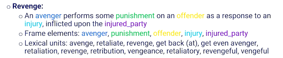
Anytime we see the concept of revenge show up, or a word about revenge shows up, we know automatically that there is an avenger who perform some punishment on an offender as a response to an injury inflicted upon the injured party. So anytime we see the word revenge we should understand that the sentence will also have other elements. There’s avenger, the punishment, the offender, the injury, the injured party, are all pieces of information we should find and be able to understand.

Also the word revenge is just one way of expressing this frame. The words that we might expect to see related to frame or that trigger this complex system of relationships come into play when we see words like avenge, retaliate, get back at, vengeful, revengeful, retaliate, vengeance. All these words trigger this notion of revenge and therefore also bring in all these frame elements as part of the understanding of how that event is happening the revenge event is happening.

So if you can identify the frame that’s at play and you can identify the frame elements then you can also make inferences between the relationships. So who was the avenger in the previous sentence about the cat? Who was the injured party? Is the avenger the same as the injured party? Who is the offender? What was the injury?

We should be able to figure out all those pieces of information once we understand that revenge is the frame at play.

Another linguistic resource, centered particularly around verbs, is VerbNet - Verbs are very important in events. All events can have a verb because the verb is the change the word that describes the nature of the change. Like FrameNet VerbNet is also manually constructed so people went through with great effort to figure out what all the verbs are in the English language and what frames they relate to and all the concepts related to those frames all written down. And what’s nice about VerbNet it also provides further information about how to find the frames and by looking at their syntactic forms.

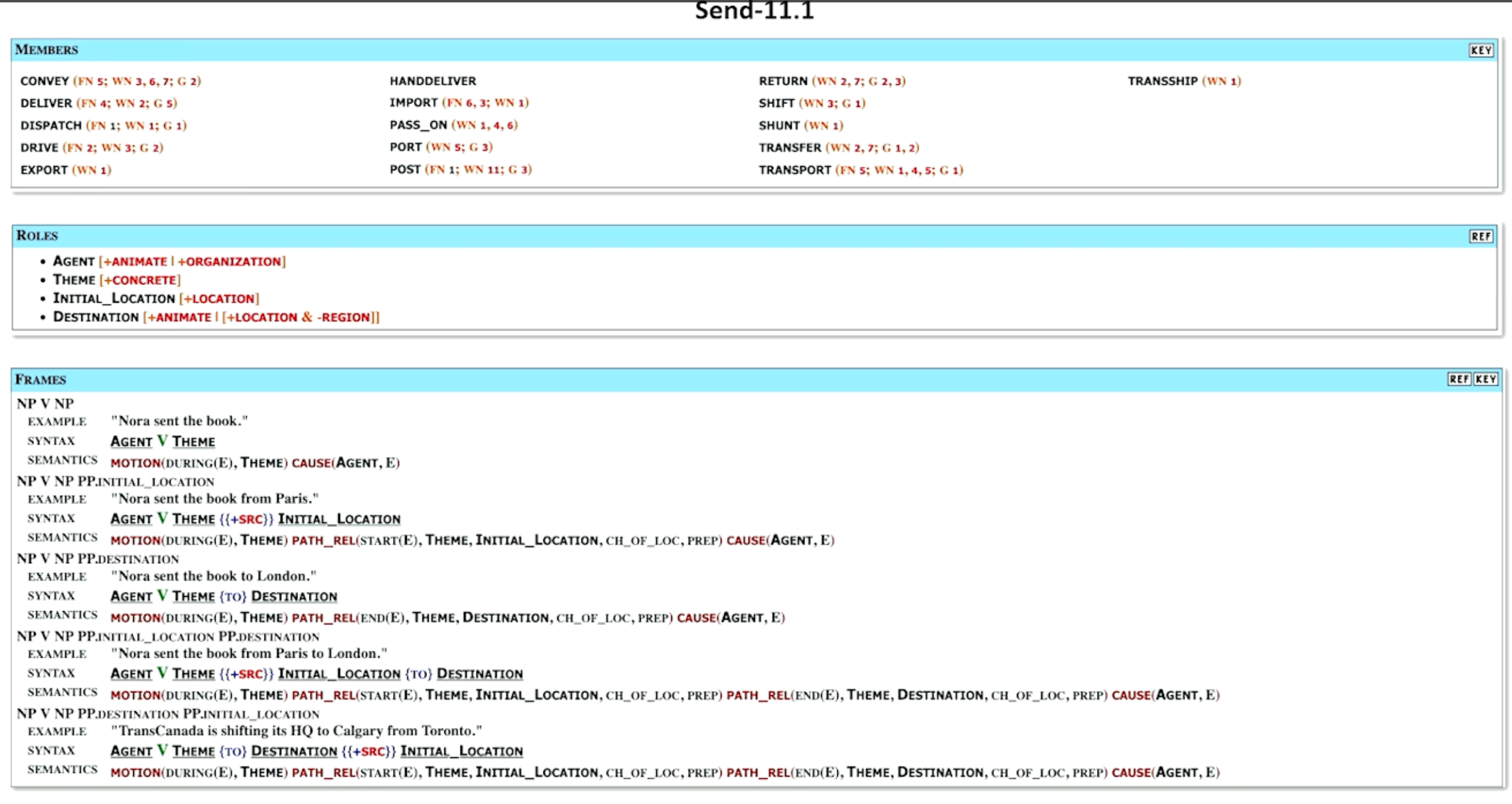
Members

tell us the different ways that we might see the verbs. So these are all verbs.

roles

If we see the send frame, or any of these verbs, we would expect to see some agent which is the sender and we further know that it’s going to be something that it’s an animate object or an organization. There might be a theme which is usually the thing being sent as some sort of concrete object as opposed to an abstract concept. We may or may not see an initial location which it will be clearly a type of location and a destination which can be another animate entity or locations as long as it’s not a relation. So this tells us the entities the frame elements just like FrameNet.

Examples

But the other thing it says is well there’s actually multiple frames associated with the send depending on how the sentence gets parsed. If we see a noun phrase and then the word send and noun phrase again for example Nora sent the book then we know that the agent is the noun that comes before the verb and the theme is the noun that comes after the verb. But if we see a noun phrase the verb and another noun phrase followed by a preposition involving a location then we also know which one is the agent is the first noun phrase. The theme the thing being sent like the book is the second noun phrase. And what comes after the preposition is probably the initial location.
It also tells us a little bit about the semantics here. So it tells us that the agent is causing the event. It tells us that the theme the book is in motion during that. So there’s some transfer of location and that there is some way of being transferred from the initial location to some unidentified final location. So it tells us a lot of extra almost logic information that we should know or be able to know just by looking at this particular sentence and the way the syntax plays out. So this is in some ways a little bit more powerful because it provides some additional information how semantics arise from the syntax.

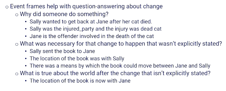
Why do we care about event frames?

Well they help us with question answering about changes. And this sometimes involves why questions like why did someone do something? Why did Sally wants to get back at Jane after her cat died? Well the answer is that Sally was the injured party. The injury was the dead cat and that Jane was the offender somehow involved in that injury. So the frame helps us with why questions.

Frames can help us with what questions of the form of necessity of change. So what was necessary for a change to happen that wasn’t explicitly stated. So when we say Sally sent the book to Jane was a necessary condition that Sally had book the location where the book was with Sally and that there were some means by which the book can transfer between Jane and Sally. And we can also tell us what things we would know that are true about the world after a change after a verb. The previous example about Sally sending the book to Jane we also know that the location of the book is now with Jane and no longer with Sally. So this frame information gives us the ability to answer these more complicated questions about relationships beyond just the factual basis.

Now of course the challenge is identifying frame challenging identifying the roles of the objects in unstructured sentences and frames and of course this is an ongoing area of research to do this particularly well. But I should also notice as we’ve noted before that these large language models are getting better and better at just directly answering questions about the roles or just going straight in answering the who what when why how questions as well.

We expect to see over time that these language models are getting better at answering questions without going through the process of parsing things out and and finding the frames and looking at frames and the dictionaries themselves. And again we’ll be looking at neural question answering as another application unit further down the road.

Summarizing everything that we’ve looked at in terms of Machine Reading.

machine reading is making unstructured text into structured tech
- usually involving factual knowledge
- but also we’ve seen event based knowledge
We’ve seen that syntax gives rise to semantics and thus gives rise to structured knowledge as well
- It allows us to do question answering
- in terms of the examples of what are facts about particular entities
- but also knowledge about change in the world that’s being described by the sentences

And at the time of recording the most robust techniques for open an information extraction are still these unsupervised parsing based techniques with little classifiers sprinkled throughout. But we do expect this to change as our large language models become more powerful and less reliant on parts of speech dependency relationships and dictionaries or frames. And again we will be looking at neural question-answering later on in a different applied section of this class.

Module 11: Open-Domain Question Answering (Meta AI)

Introduction to Open-Domain Question Answering

What is open domain question answering?

In question-answering systems we build computer systems that automatically answer questions by the humans in natural language. The open domain nature of the problem involves dealing with any questions of anything included pre-crafted knowledge bases such as DBPedia, Wikipedia concept net semi-structured information such as tables and even unstructured forms such as web pages.

There are several flavors of open domain question answering including factoid question answers which is what we’re going to focus on today. So factoid question answering is essentially questions centered around facts. Where we ask what, who, where, when, questions popularly known as WH questions. There are different flavors such as opinion questions which are centered around sentiment. So the example would be product reviews and restaurant ratings based questions. There is a third question-answering which is community QA which is often centered around quark source platforms or answers that are essentially gathered from forums, threads, conversations between human conversations.

Let’s focus on factoid question answering in this particular talk or in this particular lecture and search engines are essentially a good QA tool where we basically take a keyword as important written a web page and answer. Question-answering can be of different formats. You have multiple choice questions, span solution based questions, close questions and information extraction based question on strain where we actually glean information from unstructured sources to come up with answers.

Let’s look into multiple choice questions.

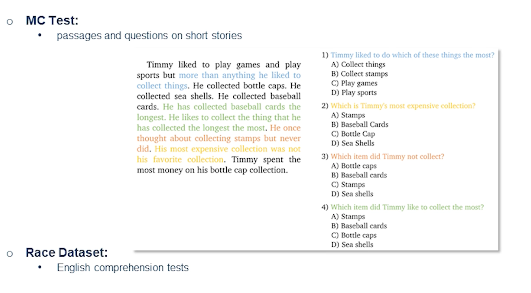
So this is an example from raze dataset which contains English comprehension test.

You have a paragraph such as on the left which says

Timmy liked to play games …. so on and so forth.

The first question is he may like to do which of these things the most? So the answer is A collect things. The answer actually lies in the sentence. However the question-answering system would look at the entire passage on the left and would be presented with the questions on the right with multiple choice answers. So the precision is key in this setting. On the other hand we have span selection based question-answering where we actually have to select the answer from extremely long passage. So the precision is key in this setting.

On the other hand,

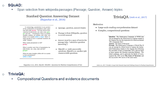
SQuAD is a Stanford question answering dataset that is a very popular dataset in this domain which includes spans selected from Wikipedia passages. The dataset is formatted as Passage-question-answer triples. The difference between them is that there are a couple of questions often that may have same answer. Unlike in the previous multiple choice questions we often see one question and multiple answers. Here the questions can be formatted in different ways where the answer maybe the same. So there are a couple of variants of the squad dataset. The difference being that SQuAD V contains only answerable questions while SQuAD V contains unanswerable questions. So when the answer itself is not present in the passage or passages.

There was another example of a dataset of this flavor called TriviaQA which is reading comprehension dataset contains over question-answering evidence triples and which is essentially trivia questions answers authored by trivia enthusiasts and independently gathered evidence documents. There are often six per question on average six evidence is per question which essentially provides high-quality distance provision for answering these questions.

Cloze

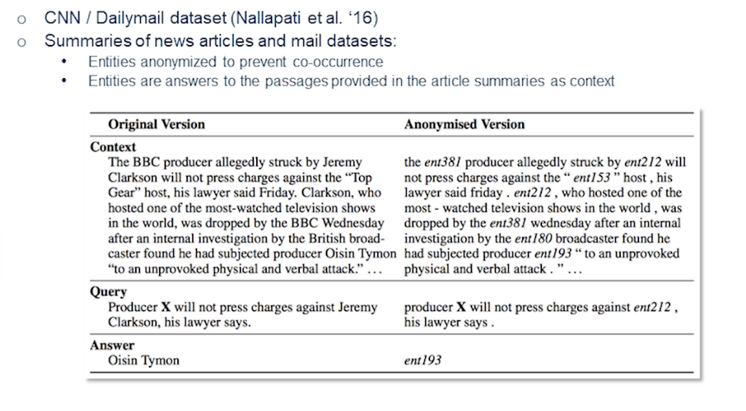
The third flavor is cloze. So CNN Daily Mail is a dataset for text summarization. Human-generated abstract or summaries are present in this dataset. The summaries of news articles and Mail datasets are present. Entities anonymized to prevent co-occurrence are essentially our answers. So entities are the answers to the passages that are provided in the article summaries.

Here’s a good example. As we see the original version contains the BBC producer allegedly struck by Jeremy Clarkson will not press charges against the top gear horse his lawyer said Friday. Now the word BBC as masked it’s presented as ENT381 and similarly Jeremy Clarkson is presented as ENT212.

So here one has to solve two problems. One is extract the entity. Which type of the entity is likely to be present in there. Now the second one would be what is the likely answer in the situation? So when we solve this problem we are essentially solving two problems which has fallen entity extraction as well as unlikely to solve the answer extraction.

Generative Question Answering

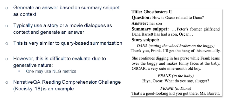
In generate question and answering (which is a fourth flavor) we are trying to generate an answer based on summary snippet as context. So let’s look into the example on the right. Here you have a title ghostbuster 2 and the answer is essentially a summary snippet or the answer itself may contain the summary snippet or in the story snippet. So typically using a story or movie dialogues or contexts we try to generate an answer and this is very similar to query where summarization.

However this is extremely difficult. Evaluate do to generate the nature of the problem. People may use several natural language generation metrics such as BLEU score or ROUGE in order to automatically evaluate these problems. Narrative QA reading comprehension challenge is a good example of this problem for dataset.

Classical QA vs Retriever-reader

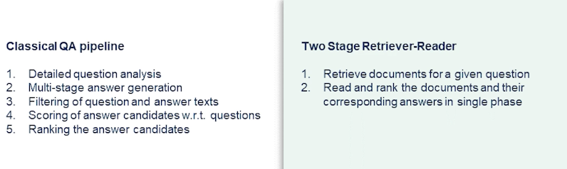
So now we have looked into different flavors of open domain question answering. So while we look into various forms now let’s look into how this problem is approached.

So first let’s observe the classic question-answering tech stack or a pipeline. Now often we have an elaborate pipeline that performance detailed question analysis. Like I said in the first slide you essentially do a WH type resolution. So I tried to identify what ATT the answer may fall under that second part of the problem. Finally you progress towards a multi-stage answer generation while filtering out question answer pays based on that relevance and importance or salients. Essentially we tried to get it the answer candidates running against respect to questions. So the final answer would have certain confidence score generated by the model. On the right-hand side we see a two-stage retrieval reader approach where you retrieve documents for a given question and go over the passages or the documents and try to read and rank the documents are the passages and their corresponding answers in a single phase. It sounds magic but it is how most of the state of the art techniques and the current day actually performed question-answering.

Retrieval-Reader

In this section we review various state-of-the-art methods that are currently approaching this problem of question answering aiming to solve this.

Input: A set of descriptive documents and a question document.
Output is an answer extracted from the descriptive documents.
- Typically Wikipedia articles are considered as the source as they often contain real world facts.

Now the framework is divided into two stages.

First stage is information retrieval stage or the candidate documents are retrieved for a given input question which is essentially treated as a query. Remember the search use case where you present a keyword and then you have list of documents it’s exactly the same.
The second phase: performs a reading comprehension stage. So the candidates are parsed for suitable our answer.

Let’s look into the retrieval phase first.

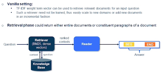
In a standard vanilla setting you would see the documents and the queries represented by their TF-IDF weight term vectors. They can be used to retrieve relevant documents for an input question. And such a retriever need not be trained so you can easily scale to near domains or add new documents in incremental fashion. That sounds easy? This is exactly the way often the most techniques are approached currently using something like a sparse vectors. And the retrieval phase could either return entire documents or constituent paragraphs of a document.

In the next phase you essentially have a set of paragraphs or sentences that are extracted that are basically saying to the extractor or the reader which computes the span of the answer, the begin and end, those positions from the sentence or the paragraphs to provide an answer.

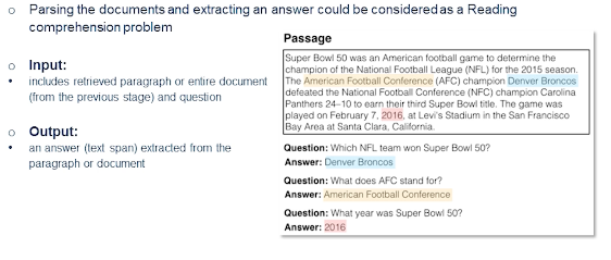
So the reader stage you’re parsing set of documents and extracting an answer. And an input in this case of course like it’s retrieved paragraph or the entire document and also the question itself. So we can look into the details how this problem is approached in the next few slides. Let’s look into the example passage here.

You can see there’s at least three answers over there and three different questions each highlighted in different colors. So the passage reads: Super Bowl was an American football game to determine the champion of the National League the for 2015 season. The American Football Conference champion Denver Broncos defeated the Nation Football Conference champion Carolina Panthers

Now the questions are

which NFL team won Super Bowl 50?
- The answer is Denver Broncos.
- In this case there is no issues of ambiguity so obviously we have a natural way to solve this problem.
What year was Super bowl 50?
- this is a much tricker questions
- this is a slightly more complex question for a classic question answering problem tech stack but this would be a very easy one to solve for latest retrieval reader-based methods.

Basic Reader Model with Document **Attention

So let’s look into the basic reader model with document attention. And this is typically how most baseline methods would operate these days for question answering on the reader side. You have a document or a passage, let’s imagine this is Wikipedia document, and then you have a question around the entities present in that document. Now we encode both of them and they are positive pairs by the way. So let’s say this is given the training data. So this is further encoded in a joint latent space. And now the idea is to provide how the answers are generated but essentially allows us to fine tune the question answering datasets.

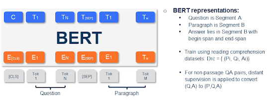
As you probably know that what is a transformer-based method which essentially allows you to fine tune to target task. So we can perform fine-tuning for question answering task where you would like to consider the Segment A that is right after the CLS a special token as a question and you have a separator token. And then you present the paragraph which is essentially where the answer lies. The output of such an approach would be the answer where you basically provide the span that is begin and end of the answer in the paragraph segment. What most reading datasets would include is a triple so you have a question then you have a paragraph or a passage and then you have the answer.

So that is how typically reading datasets are used for training. However there is a chance that you do not have a paragraph you simply use question-answer pairs. So now you’ll have to use something a technique called distant supervision where you convert the pair into a triple. So one may choose to query or use the question has a query and potentially pick several passages or paragraphs and then maybe use all of them as their positive examples. And some may be negative examples too but this is considering this as a silver dataset one would consider training on this dataset. And potentially multiple passages may have the answer so that’s why we need to consider a second phase ranking. So we’ll go more into the details of how reranking and other things will work out later in the lecture.

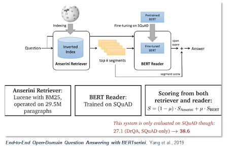
So this is a very popular framework called BERTserini which is based out of previous slide where we discused how we could apply BERT to this question answering task. So here the retriever is responsible for selecting segments of texts that contain answer which is then passed to the reader by answer span. So the single-stage retriever in this case tries to identify segments of texts from Wikipedia so that we can pass it to the BERT reader as opposed to a multi-stage read retrieval. Where we first retrieve your documents and then rank passages within and so on and so forth.

So this particular approach has tried to index different granularities of the texts. By what I mean is you could either index the articles, or you could index the paragraphs, or you can index the sentences. While at the inference time you retrieve the segments either it can be paragraphs intense or articles using the question as a bag of words query. So this is basically a BM base retrieval which was previously covered in the information retrieval lecture. Next segments from the retrievers are then passed to the BERT reader. So this is the model that is the vanilla BERT model that was proposed by Devlin et al. in 2018. But there is one slight difference which is to allow comparison and aggregation of results from various segments. So basically they remove the final softmax layer over different answer spans.

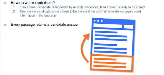
Now we talked about reranking and that’s actually a very important step when you actually have multiple paragraphs or passages or even long documents. It’s extremely impossible or could create latency for the second-stage reader to actually look into every passage that are retriever returns. Instead people have approached this problem using something called passage re-ranker where you only return both passages or performance against the ranking where you actually just look into the candidates that are likely to have answers.

Training Methods

In this section we will deep-dive into several training methods that have been successful in open domain question answering. So we will advance through some of the more latest techniques.

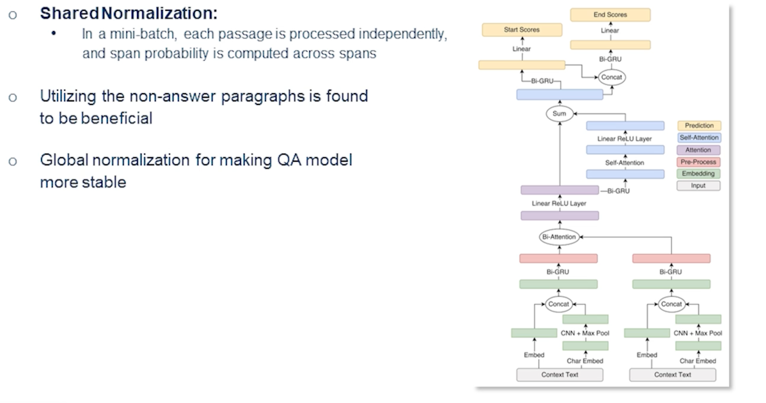
Let’s begin with multi-passage training. Often the problem is that we utilize just one passage but we could use multiple passages at the same time. And often the non-answer paragraphs or the passages can be extremely beneficial. If you see on the left-hand side so one of the context in this case certainly a paragraph that doesn’t have an answer but also help towards identifying the answer. And the global normalization actually makes the question-answering model more stable while pinpointing answers from large number of passages.

So if we could split the articles into different passages and put them into a mini-batch and each passage is processed independently and we compute a span probability across various span that will actually make the performance of the models that much more better. And there is an existing work which actually showed this: BERT-based passage rankers actually give 2% more improvement over the previously looked at BERT reader that we have seen.

However there is one caveat sometimes the explicit sentence-level matching may not be quite helpful.

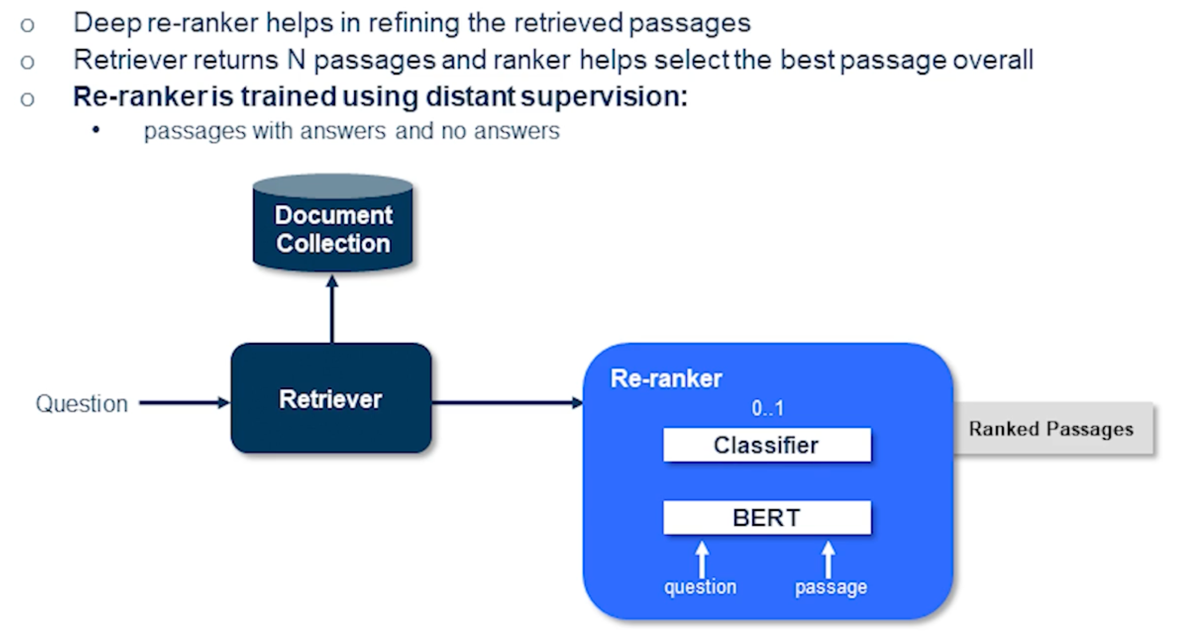
So in order to address that issue often it’s good to have this re-ranker phase where we explicitly pass the question in the passage and train a classifier essentially a second stage ranking where you have a way to say binary classification this is a right passage or a wrong passage for a given question. In this situation we actually get a series of ranked passages and most of the positive passages were likely to be end up at the top of the list.

Several methods are actually employed this deep re-ranker to refine the retrieved passages. There is a recent work which actually as simple as this technique that I’m showing here it simply computes the probability for each passage independently and obtains the final list of passages.

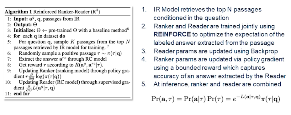
There is a little more advanced technique than the previously seen one. This is a joint training of the reader and the ranker where we have an information retrieval model which retrieves the top-n passages conditioned on the question. And then you have a ranker and reader which are trained jointly using reinforcement algorithms to optimize the expectation of the labeled answer extracted from the passage. So while the reader parameters are updated using a back propagation, ranker parameters are updated via policy gradient using a bounded reward. So one could think of the ranker has higher honors of actually getting the right answers from the correct passages. Rather correct passages being ranked on the top and the poorly or negative answers or passages with no answers would be ranked in the bottom.

So the inference ranker and reader are optimized in the following fashion. So with this actually one could apply this model to any of the retriever approaches irrespective of whether it’s a dense retrieval or a sparse retrieval. We’ll go more into the detail of the retrieval phase later on. So when we’re talking about the retrieval I said sparse and dense retrieval.

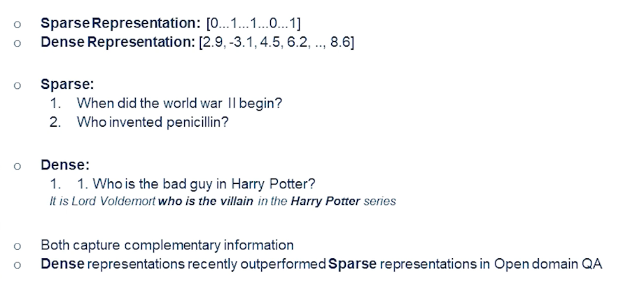
What does sparse retrieval mean?

So when we look at the example at the top of the slide we are essentially denoting every token that is in a question as whether it’s been present in the index or not. So we are essentially saying there is a token there’s no token and so on and so forth. That’s a sparse representation. And in dense representation obviously we know which question contains what kind of words in there in the cancelling words and then we basically come up with a word vector or a sentence vector and so on and so forth. There are various ways to come up with a dense representation in a distribution semantics way.

So when we look at the sparse representation not all words in the question need to be in the index. So when I say index it’s basically the training data or non-training data but how we indexed the initial set of documents in our database and then we compute some scores around them using TF-IDF or some other similar techniques. And then basically assign certain score to every word that’s present in the index. And then basically the inference time you’ll end up with a sparse vector.

Whereas in a dense retrieval or a dense representation we have a way to ask more complex questions such as who is the bad guy in Harry Potter? And the answer can be pretty complex. In this case it is Lord Voldemort who is the villain in the Harry Potter series and so on. So it’s not like the dense retrieval is better than sparse retrieval they actually capture complimentary information. And only recently we have seen dense representations outperform the sparser representation in open domain QA.

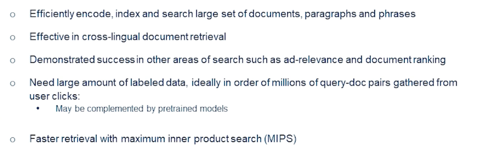
What are the characteristics of the dense retrieval and why do we need to use dense retrieval? Sparse retrieval is often based on simple term matching which is obvious limitations. Latent semantic encoding is complimentary to sparse representations by design. So for example synonyms or paraphrases that often contain completely different set of tokens. So they need not be in the vocabulary of the index. So at the time when you’re creating the index or the database those words may or may not occur. Whereas in a dense setting and that is not at all a limitation. It’s okay to not have those words in the vocabulary at the time of indexing. Instead you’ve leveraged the fact that there are computing vectors that are likely to be similar based on their synonymy or if they’re paraphrases in case of sentences and they could altogether contain totally different tokens. And sometimes people have also utilized different languages cross-lingual documents and they’re still effective. So the words that are likely to be translations in different languages would end up having somewhat similar vectors in the close neighborhood.

So basically term matching is good enough for extremely well understood domains. Whereas dense encodings can be very interesting and they’re also trainable and they will provide additional flexibility when we have task-specific representations or domain-specific representations or even sometimes the languages do not have enough vocabulary coverage to begin with. And again all of these methods both sparse and dense can be equally useful and some of the times I think dense is more preferred. As I said it can be pretty easily deployed in an index. And we can use maximum inner product search to compute nearest neighbors vectors. So a query is represented or encoded as a vector and then it retrieves a series of documents using this fast nearest neighbors research rate.

Recent Approaches in Dense Representations

There are several recent approaches for dense representations such as

ORQA
RAG - Retrieval Augmented Generation
REALM and
DFR - Dense Passage Retrieval.

Let’s go through each of these techniques and discuss some of their advantages and disadvantages.

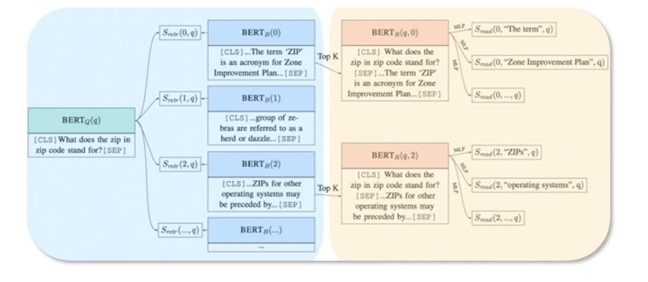
ORQA is a model that was introduced by Lee et al in which was one of the first methods Stuart performed BERT for open domain query. Until then most often people would have used BM25 in the retrieval. And mostly the innovation has happened on the reader side of things. So ORQA would actually propose this an inverse close task objective which various blocks that contain the mass sentence and thus contains an additional expense of pre-training step. And the context encoded is not fine tune using pair of questions and answers. And the corresponding representations could be sub-optimal in that case.

So it has its own advantages and it has been found that it’s necessary that we augment the retrieval with generation. That is to say that it is good to have a generative way to predict what tokens smart likely to occur. And then in an answer or even in a question for example there is certain way we can parameterize this.

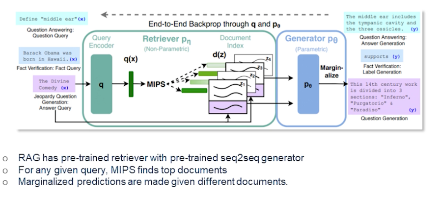
So here comes retrieval augmented generation which actually trains the Retriever and a generate end-to-end and treats the retrieved documents as latent variables. So basically there are two models that marginalize over in documents in different ways. So the paper from Louis et al. in 2021 which actually proposes two slightly different variants of the RAG architecture. more details are in the paper but here I’ll give you the overview.

Basically the RAG sequence there is the model actually uses the same document to predict the target token and that is the second variant which actually the rack token which predicts each target tokens based on different document. So in the first setting the RAG sequence uses the same document to predict target token which is likely to be an answer. And the second approach uses each target token based on different documents. And finally the Retriever competent in either of these variants is just a by encoder architecture and the generator component is based on the BERT which has a generative model for denoising autoencoder model for generating text. Ideally any generator could be used in this case and that’s how it is currently set up in the RAG.

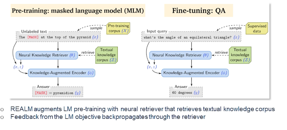
REALM is another technique that augments the language model pre-training with the neural tube are very similar to RAG in that sense. Where the feedback from the language model object to backpropagate so the retrievers here the presentations are pre-trained to perform reasoning over a large corpus of knowledge on the fly and explicitly exposes the word knowledge thus the model could use to retrieve and at the time of interests as well. The language model uses the Retriever to retrieve documents from a large corpus like Wikipedia or even the glue web or other open web documents. And then it ends over the documents to help through during the prediction time.

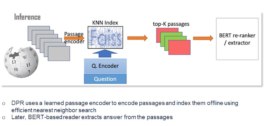
DFR (Dense Passage Retrieval) As we are talking about different retrieval and reader techniques this is primarily an interesting retrieval technique which essentially does a learn passage to encode passages and index them offline and then apply MIPS or any other efficient nearest neighbor search. So later on then we have a bird base reader which exact answer from these passages. At runtime obviously a question comes in and then you construct a vector out of it in the same latent space and then you select the passage itself which vectors are close to this question. And the BERT based answer extractor is essentially going over the passage and figures out this time span. So the main contribution of this work is that the retrieval part could practically be implemented using dense representations are known. And actually this was the greatest advantage over BM25 like methods which are sparse retrieval methods and which actually was found to be a new state-of-the-art on several benchmarks.

Multi-Hop Reasoning

As we progress into various retriever reader architectures one may see that question-answering is always about: a stiuation where we have several passages, one question, and then we figure out which of these passengers may have the answer and then we discover which is the right answer.

What if there are several series of questions and the questions are connected to each other and answers cannot be retrieved in one shot? Then we need to have multiple hops in this situation. What do I mean by that?

Let’s focus on this example;

Jack went up the hill
Jack put down the pail
QUESTION: Where did he put the pail?

Now the last question or the last statement which is actually the question need to be addressed in multiple ways. First we need to know what does the pronoun “he” referred to. So in this case it should refer to Jack. And where did he put the pail? Now that’s the question where we need to understand that he went up the hill and he put the pail on the hill.

So this problem is known as multi-hop reasoning and multi-hop question-answering is an extension of it. So information that is presented in a post facto way and then there are multiple datasets that are created through multiple steps. The most prevalent one in this setting is hot pot QA and there is another previous dataset which has a fixed number of sequences which was a precursor to the hard part QA.

So what really changed when we do single-hop versus multi-hop?

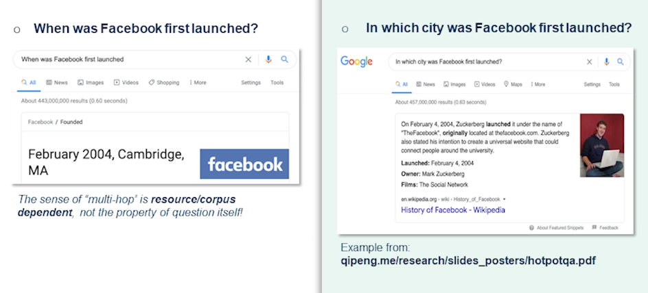
Let’s look into this question.

QUESTION: When was Facebook first launched?

The answer could be straightforward. In this case February 2004 Cambridge, Massachusetts. Whereas when somebody asks them the right-hand side in which city was Facebook first launched? So this would require it’s not explicitly answered in a single Wikipedia paragraph where it says on February 4, 2004 Zuckerberg launched it under the name of “the Facebook” originally located at thefacebook.com. Zuckerberg also stated his intention to create a universal website and so on and so forth. That actually doesn’t have the immediate answer. So this is actually a good example of how the city needs to be figured out.

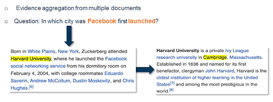
So when you look at the actual paragraphs we find there is additional evidence from multiple documents which actually says where was Zuckerberg born and where did he attend the university. So one would know that Zuckerberg was born in White Plains but that’s not the relevant information here. He attended Harvard University and where is Harvard University located? Its in Cambridge Massachusetts.

So the answer indeed is in there multiple pieces and retrieval needs to retrieve both documents and most of the time the documents need to be retrieved and sequence. Since you need this information in the first paragraph to retrieve the second paragraph this type of question is sometimes referred to as bridge questions and the intermediate information as bridge entity.

Existing Solutions for Multi-Hop Retrieval

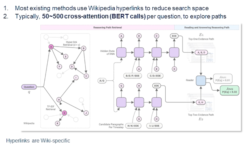
So there are several interesting solutions for the multi-hop retrieval. The challenge for multi-hop retrieval is actually the search space of candidates, where the candidates of chains where the documents grow exponentially at each hop. Almost all existing work make use of Wikipedia hyperlinks to narrow down the space and these chains are restricted along the edges of the hyperlink graph or the Wikipedia documents. Obviously this approach would generalize or may not generalize depending on the domain. We cannot simply rely on the hyperlinks.

Let’s take an example sometimes the medical documents may or may not have enough hyperlinks. In general the web doesn’t necessarily connect all the relevant webpages from a given webpage that is through hyperlinks and moreover such approaches can be too restrictive. So in that sense that’s why hot part QA was created as a data set where we could sample them just across the hyperlink graph and then generate the questions. And this is not exactly sufficient to narrow down the search space. Again the tough methods need to rerun 50-500 chains in doing expensive cross intention computation for each candidate.

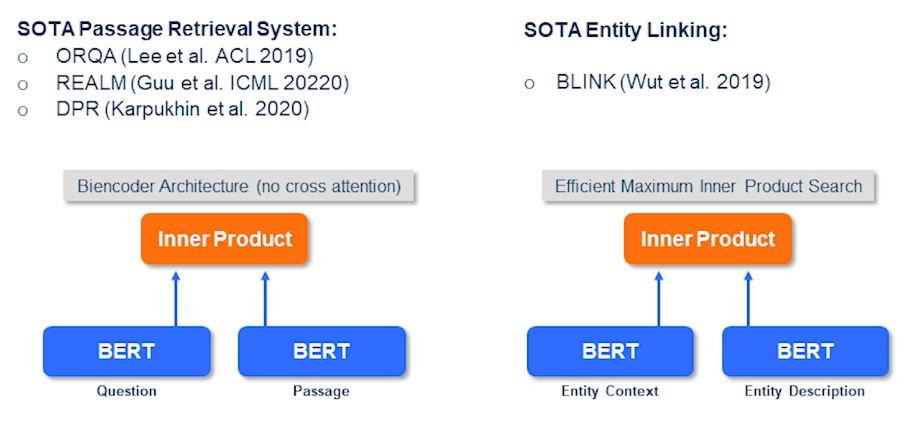
So here are some other methods. Like I previously discussed you have to perform passage retrieval which can be done in several different ways where you can apply a by encoder architecture with no cross indention. Then you were to let’s say perform state of the art entity linking using blink and similar techniques. So where you have an entity of context and then you have an entity of description and you perform inner product between them.

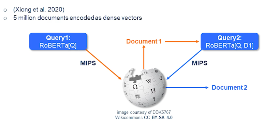
So here comes a very interesting technique called multi-hop dense retrieval which essentially is a very simple technique if you look at it. So firstly income subquery and you have a RoBERTa which is a flavor of BERT. So it actually encodes the query and performs a search on an index of vectors that are trained and encoded passages from Wikipedia and outcomes of document 1. And now you run a second round where the query or the question includes the original question queue and also the document D1 which is the top document. And then we again perform a second search where outcomes the document D2. So in this way we could perform multi-hop dense retrieval and this is how mathematically it would look like.

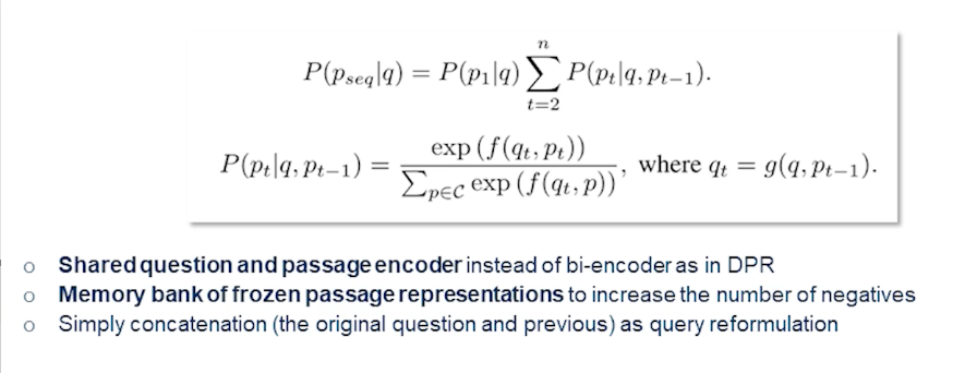
It’s always measuring the probability of sequence of passages given the query and now once we have the first passage given a query then we break it down into a sequence of passages that are given the previous passage and the original query itself. And then simply compute the probability. How likely it would come the current passage would come out to be the best candidate given the query in the previous passage. So the shared question and passage encoder instead is preferred over by encoder as in the DPR and memory bank of frozen passage representations will also increase the number of negatives. And simply concatenation of the original question and the previous one as we see is used as a query reformulation.

Datasets and Benchmarks

In this section we deep dive into some of the datasets and benchmarks that we could apply to various approaches that we have discussed in the last two sections.

Let’s begin with some of the datasets that are popularly used in question answering.

bAbl is an automatically regenerated synthetic dataset such that a model can learn characteristics of a language
- it’s a very simple dataset.

Another one popularly used for benchmarking question-answering system

Natural Questions, which are questions are created from search logs using crowd workers to find corresponding evidence for a given answer.

there are more well-curated datasets such as

TriviaQA, mentioned in the previous slide.
- Reading comprehension with complex compositional questions
- text evidence is based on the web-search queries.
SearchQA
- where the QA pairs are based on Jeopardy Archive
- The search queries provide text evidence
Quarsar-T which is trivia questions
- based on searching and reading the Clueweb
- which is probably a subset of the overall Clueweb09, which only contains one billion web pages.

HotpotQA and FEVER which are essentially multi-hop and multi-evidence datasets

HotpotQA actually includes natural multi-hop questions with some supervision from supporting facts
- thus basically leading into explainable QA.
- questions require finding and reasoning or multiple supporting documents
- question are diverse in nature and not constrained to any pre-existing knowledge or knowledge schemas. And there are sentence-level supporting facts required for reasoning and so that QA systems could reason with strong supervision per se and explain the predictions as well.
FEVER is another dataset
- which has essentially a fact-checking algorithm sentences dataset.
- assume that we look at Wikipedia paragraphs and we modify some of the keywords usually. Thereby you’re creating misinformed paragraphs in a way. The claims in this case so the paragraphs are with certain information in there could either be considered as supported, refuted, or not enough info if they’re too ambiguous because we modified those sentences.

So thereby each of these datasets are pretty relevant for multi-hop and multi-evidence question answering systems.

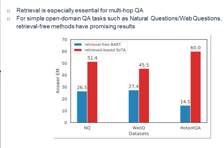
So in a typical multi-hop question answering system the retrieval could be as simple as looking at state-of-the-art methods. We could also use similar techniques that we have used in a single hop setting. So they still fall behind as you can see in the natural questions and web questions which are single hop set the methods not necessarily have a advantage when they don’t have the generative power. So the techniques that we are discussing here are primarily like say the techniques that do not use a generator towards the end. So something like BART. That’s one reason why retrieval is actually more crucial for this multi-hop question-answering.

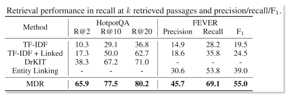
So as we discuss the multiple density we’ll actually is much more performant in the situation because of the nature of the approach. Where we see the crowdsource questions from HotpotQA are fact-checking datasets such as multi-a and like a fact-checking datasets such as a FEVER we see that strong results techniques are TF-IDF and entity linking baseline. That’s the interesting part. So here we’re measuring the precision and recall, as well as the F_1 score.

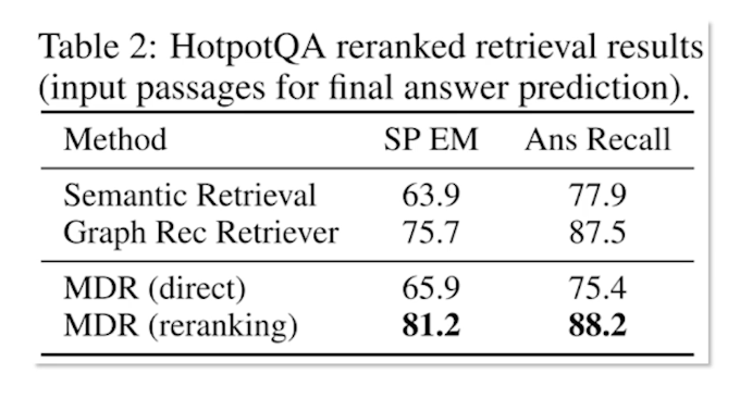
One could actually argue that the ranking itself is not sufficient. Especially when you are looking at multiple documents you may need more evidence when you gather more documents. So in that effect obviously reranking actually helps. So retrieval results offer cross attention reranking compared to not reranking. That is simply doing the direct just one short retrieval and ranking is actually no good.

So as you can see there is nearly 10% absolute improvement on that inversion absolute improvement in the recall and nearly 15% absolute improvement in the exact match. So exact match meaning the answer exactly matching the ground truth. Similarly the previous state of the state-of the-art methods such as graph retriever would also stand no chance with the MDR approach. So it helps to have this cross attentionary ranking in this kind of multi-hop setting.

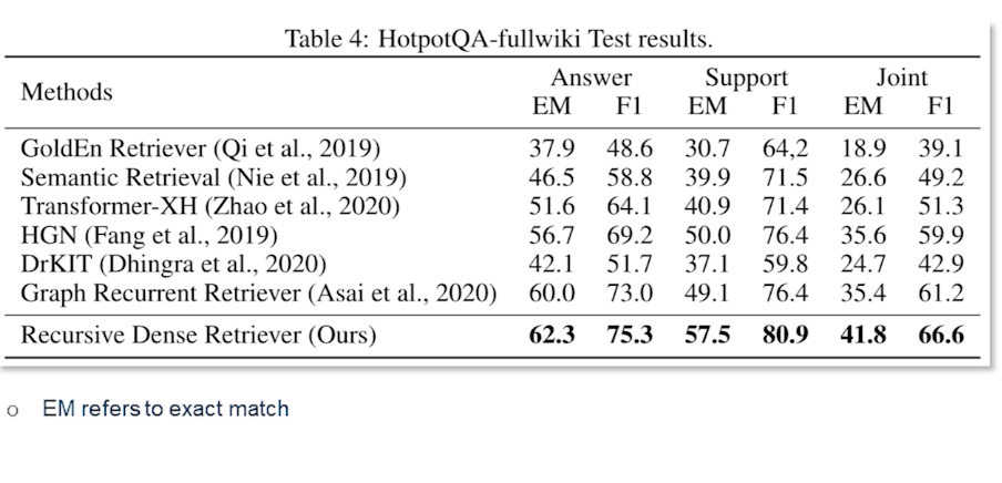
Furthermore as we see the Recursive Dense Retriever actually does perform much better than the other retrieval base methods. And you can see that exact match is prominently higher against the competing methods. So similarly for the F_1 score especially for the evidence and also combined answer and support together is also very high. It definitely shows that we have more scope for retrieval in multi-hop setting as opposed to in a single hop setting. That is to say one must pay more attention to what documents are being retrieved and thus they need to be reranked more often in order to get to the actual answer in a multi-hop setting.

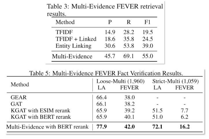
As you can see similar story can be told from the FEVER fact verification results. So almost by points the strict multi-evidence set performs much better than the nearest previous state-of-the-art method. This indicates that multi-evidence and multi-document or multi-hop retrieval and reading is essentially a very promising direction in the open-domain QA and soon it becomes even more an interesting challenge as there will be more such datasets similar to a HotpotQA and FEVER.

The main takeaways I have from this lecture is that

Open-domain QA has several flavors
Often Reader and Retriever base methods is the go-to framework as of now.
Simple efficient pipelining approach has outperform complicated pre-training end-to-end schemes. So we need techniques that can be optimized and obviously that are fast enough for specific domains.
But again there are certain limitations like bi-encoder optimization is challenging while it provides value.
Dense retrieval is faster and better

Module 12: Machine Translation

Machine Translation

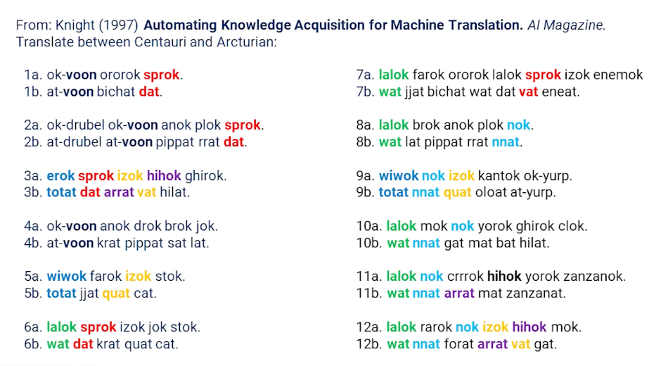
Some words are repeated / observable patterns - even as we see across multiple different phrases. This gives us hope that we might actually be able to do machine translation without really even truly understanding what language means.

Examples of machine translation efforts past the years:

World War II code breaking efforts at Bletchley Park , England (turing)
1948, Shannon and Weaver information theory
1949, Weaver memorandum defines the machine translation task
1954, IBM demo, 60 sentences from Russian to English
1960, Yehoshua Bar Hilel suggests that high-quality MT will require the understanding of meaning.
1966: Alpac report comes to the conclusion that human translation is cheaper & better than MT research
1990: IBM CANDIDE - the first statistical machine translation system
2000: Progress in statistical machine translation and phrase-based MT
2010: Neural Machine Translation

What exactly makes translation hard?

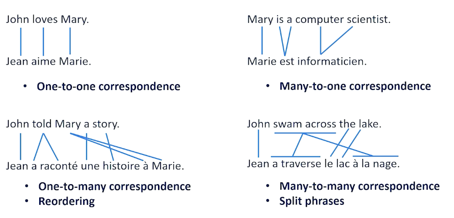
one to many correspondence or many to one correspondence or even many to many re-ordering of words
split phrases
different word senses
- in english we have river bank and financial bank, but in german they have 2 different words for such nouns
- in english we just have brother, but in chinese older brother is (gege) and younger brother is didi
Word order
Head Marking vs Dependent Marking to indicate possession.
Gendered words
Pronoun dropping
Negation

Machine Translation Background

Suppose you had a “perfect” language that could express all thoughts and knowledge
Maybe it is first order logic (or maybe not)
May need more information that your representation cannot express
Hard to think of semantic representation that covers everything
Maybe if all languages have the same semantic ambiguity then our representation still works
Not true for all languages

The vanuquois triangle

The concept of having a perfect language is still useful to think about and it’s useful to think about in the following way. So we think often about something called the Vauquois triangle.

This is a way of saying how do we get from a sentence in a source language to a sentence in a target language? Well we want to still think about this as being able to go to some perfect language in the middle through a process called analysis.

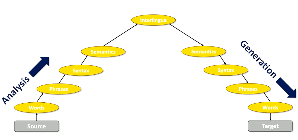
We want to take that source we want to break it down into words
analyze it at the word level, then merge the words into phrases
analyze things at the phrase level
look at the syntax relationship between things and the phrases.
We also look at it at the syntax level look and the semantics level.
if you do this analysis long enough you would get to this perfect language: Interlingua

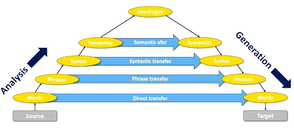
Now the reason why this is a useful thing to look at is because when we set it up as a triangle like this we might think do we really need to go to the interlingual? Maybe we can do something called transfer maybe I can stop my analysis at the word level and try to do direct transfer to my target words so word to word translation or word to word transfer. Maybe I’ll allow the analysis to go to the phrase level but I’ll try to translate or transfer phrases into my target language. Maybe I can go all the way to the syntax level and take syntax trees and syntax analysis and what we learn in that process and transform it into syntax. And maybe we can even do this at the semantic level.

The point here is if we’re never going to have this interlingua then we need to find a way of short cutting across this triangle. And to do that we have to pick the level of analysis we want to work at. Let’s look at some examples of what language translation looks like when we start thinking about it as transfer. So direct transfer is basically word to word.

Here’s an example of Spanish to English

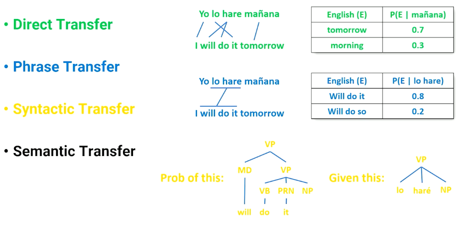
Word Level you can actually see some re-ordering here. But if we’re going to treat this as a direct transfer word to word we would get a jumbled sentence that isn’t quite fluent English. But the point is if we just go word through word there must be some way of making this translation happen maybe a statistic. We might say there’s a probability that we see the word tomorrow given the word manana and there’s a slightly less probability that we see the word morning given manana. So we can just maybe take the most probable translation based on some statistics about how languages relate to each other and we’re good to go we have direct transfer. So that’s word level.
Phrase level well now we want to do a little bit better. We want to recognize that phrases like lo hare tend to translate not word by word literally, but to chunks of English. So there’s some probability that lo hare should be replaced by “Will do it” and some smaller probability that it should be replaced by “Will do so”. Although both are somewhat reasonable.
Syntax Level can’t be expressed as a nice probability tables anymore but you have some syntax structure for lo hare and the noun phrase that comes after that. So what is the probability that the simple verb phrase that we see in Spanish would look like a more complicated, in this case syntax tree, that happens in English? Are these things probabilistically likely to be interchangeable? And we’d need to build statistics on how trees relate to each other in syntax transfer.
Semantic Transfer We don’t have an exact example of this because semantic transfer isn’t done very often and I think we’re still figuring this out but you would imagine that you can look at things at the semantic level as well.

Now we have a bunch of probabilities. It would be useful at this point to step back and remember Bayes probability rule.

Recall the bayes formula: $P(x \lvert y ) = \propto P(y\lvert x)p(x)$

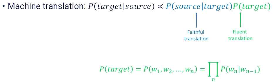
P(source $\lvert$ target): correlates to a faithful translation
P(target): is the fluent translation
- the reason why this is nice is because they mean something very specific that we can understand.
to understand fluency we look at an equation we’ve seen many times
- $P(target) = P(w_1,…,w_n) = \prod (w_n \lvert w_{n-1})$
- We break the target down into words and we can compute the word given its previous context.
What this tells us is there’s a language to language probability.
Any good translation will also look at that target and say whatever we translate to are we likely to see this as a plausible sentence in the target language? So we want both of these things and the statistics are going to give us that.

The faithful translation is the tricky part here. How do we know the probability of a source given a target? Well we have a clue how to do this and this clue is something called parallel corpora. We want to find this parallel corpora that tell us the exact same information in two different languages side by side meant to be faithful to each other. So the two documents should say have the same meaning but be in different languages. And the place that we find a lot of parallel corpora is

in legal and parliamentary texts from languages that are multi lingual.
- think European Union where every legal document in every language must be translated to every other language in any country in the European Union.
- Canada is another example where French and English are both official languages so everything that’s official has to be given in both languages.
It turns out there’s lots and lots of parallel corpora in the real world and we just have to find that and make use of it.

A parallel corpus looks like a collection of sentence pairs. We might see the English and the Spanish side by side and we would basically know that each of these phrases were equivalent to each other. And now because if we know English or Spanish but not the other one we actually understand what’s being told to us and we can look at how it’s being expressed in the other language.

Evaluating Machine Translation

How do we know a Translation is good? Well in machine translation there’s really kind of two phenomenon that we really care about.

Fidelity. Fidelity means does the translation capture all the information in the source? That is if I tell someone one thing and I tell another person something else with a translation have I given those two people the exact same information?
Acceptability So acceptability is asking whether the translation captures enough of the meaning of the source to be useful. So this is an argument to say that translation doesn’t have to be perfect to be useful. It’s not perfect it’s not fluent but it’s acceptable.
Acceptability is a spectrum, Fidelity is much more binary, You got all the information or you didn’t

If we had a machine translation system the gold standard would be human evaluation. We would put the originals and the translations in front of people and we would ask them either to judge the fidelity or to judge the acceptability. But humans are expensive! We would rather have some automated way of doing this. Preferably mathematically,

Machine translation makes use of a number of automated metrics. BLEU score being the most famous.

BLEU: Bilingual Evaluation Understudy
- the geometric mean of 1,2,3, and 4 gram precision multiplied by a brevity penalty
- the geometric mean might favour short translations which might mean the translations are dropping information
- so we then penalize things that might be too short

We would also need a corpora, here are two potential translations

Maybe this means both of those to some degree.
Now let’s suppose that our Machine translation produces three possible translations (hypothesis)
How do we know whether one is better than the other?

So the first thing we do is we look at the geometric mean. At each of the 1-gram 2-gram 3-gram 4-gram so on and so forth. I’m just going to go up to the gram level but we can basically look at each of these hypotheses and we can go through the different grams.

Hypothesis 1
- we see there are three 1-grams and each of these 1-grams appear somewhere in one of the references. We don’t care about ordering but we see I, am, and exhausted in both of the references. So we get 3/3. At the 2-gram levels there’s only two 2-grams that are possible. “I am” and “am exhausted”. Further, only “I am” shows up as a 2-gram, a bigram, in the references. It shows up twice but we only get one point for that so we get one of two bigrams show up in our references. There’s only one 3-gram none of which show up exactly in the reference. We get zero there.
Hypothesis2:
- if we do case sensitivity in this case we’re doing that we see only one -gram that shows up in the reference I. We see none of the bigrams show up and the trigram doesn’t show up at all.
Hypothesis 3
- we do see one of the 1-grams show up tired tired is in the references it’s repeated but we don’t care about that. We just see is it present or not. None of the bigrams and none of the trigrams. Then depending on how you do smoothing and some of the other things you come up with a geometric mean.

You might come up with something along the lines of hypothesis 1 having a very good geometric mean score, hypothesis 2 having somewhat less and then hypothesis 3 also not particularly great. Again don’t get caught in the numbers. I don’t remember how I did the smoothing to come up with these numbers. The key is that what we’re already seeing right now is that hypothesis 1, the one that we intuitively think is the best one here is in fact showing up as having the higher score.

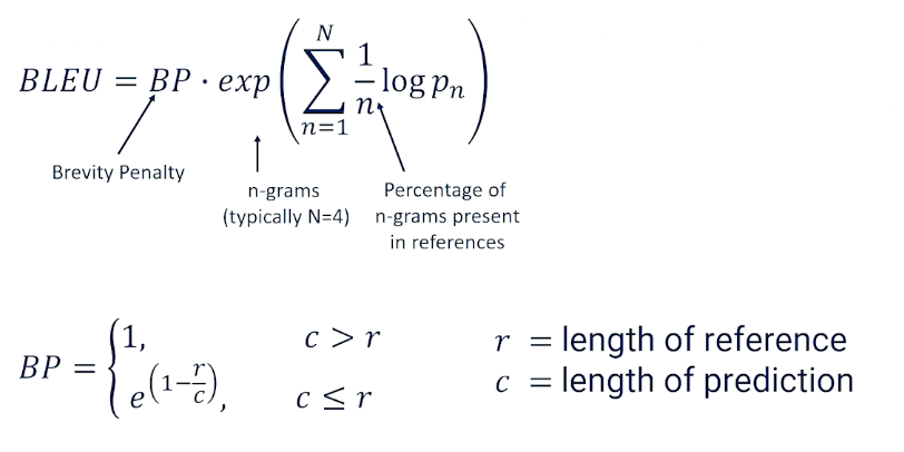
So the complete BLEU score is calculated as the geometric mean times the brevity penalty. For the penalty term, If you have a very short translation you have a lot of 1-grams but maybe you don’t have a lot of 2-grams and 3-grams and 4-grams. The geometric mean is going to be quite okay with that. But we want to basically make sure that we come back in and say well hold on we don’t want to just say “tired”. We don’t want that to come out as seeming like good translation. What we do is we say if the length of the prediction is greater than the length of the references we’re fine. The brevity penalty is just . There’s no penalty. But if our length of our predictions are smaller than the reference then we apply this penalty here to make sure that we are not giving an artificially high BLEU score for basically translations that are likely missing a lot of information just because they’re way shorter than what we should expect to see with a good translation.

These two components go together to give us the BLEU score. Again this captures the intuition that the translation is somewhat faithful if not just acceptable.

Machine Translation as Transfer

We’re finally ready to talk about machine translation as transfer. We’ll do so at both the word level and the phrase level in this segment.

Recall that “direct Transfer” is word-to-word, so word level. So machine translation via direct transfer will also be word to word. Just as before we will run into some word ordering issues.

Glinda no dio una boftada a la bruja verde (in spanish)
Glinda not give a slap to the witch green (to english via direct transfer)

To get around direct transfer issues is we go to phrase transfer, which is where we’ll spend most of our time. Recall from our seq2seq models

Transfer works better when we’re dealing with larger chunks of text. Often chunks of text in one language, ie phrases, seem to translate naturally to other chunks of text.
So to do phrase transfer, we just need to figure out what these common phrases, aka chunks, are and stich them together

The Stitching is the most challenging

first is what are these common phrases?
How do we identify these phrases? How do we do word alignment within these word phrases?
And then how do we stitch these phrases together?
- The fluency is going to be very helpful in terms of stitching as we’ll see.

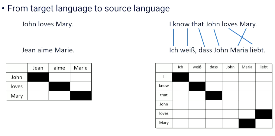
So if we want to figure out which phrases are going to be the ones that we have to remember and keep track of because they translate well to each other. We need some way of figuring out which are these word phrases that we should keep track of irrespective of their word ordering. So we’ll look at two examples here. The example we saw before which was John loves Mary going to French. And that was an example that we saw where there was no word ordering issues here. This is the straightforward thing and we know it’s straightforward because if we plot this along a matrix. We can see every single word maps to the next word in particular order and we get this nice diagonal. So first word goes first second goes second third goes to third. That’s what that is telling us.

Compare this to something that has not so literal word alignment. So I know that John loves Mary has some word re-ordering issues here. So I know that those words are in order. But then we see the swapping of loves and Mary shows up as a different pattern. So we see the diagonal break. So what we want to do is we want to find a way to identify the fact that this is a chunk that we should keep track as being separate. Whereas all the other words we can deal with on a word to word basis.

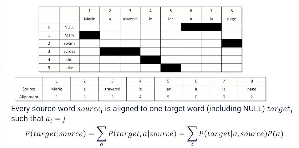
To do word alignment, we’re going to make one small change to this diagonal alignment chart. We’re going to add the null because we want to sometimes recognize the fact that some words just don’t show up in the translation. And this allows us to basically go through and find a mapping or an alignment in terms of word order.

In this case Mary is the first word maps the first word. But then we have the second word becoming the third “a traverse” seems to go together. So the third words maps to the third word as well four to four five to five six and seven don’t show up in the translation at all. And eight the eighth word is actually referring back to the swimming, the swam word. So this is the alignment chart and what this allows us to do is basically keep track of the alignment. Every word source sub I has to be aligned to one of the target words. Including null target j such that $a_i= j$. That’s just telling us what this thing is telling us here. But once we do this we can make a small update to our statistical math. We can say the probability of a target phrase given a source phrase, now should be the sum across all possible alignments of the target and the alignment given the source. So we’re adding a in here and what we’re basically trying to do is say now we have to go from source and predict not just the target words but also the alignment as well. The for example needs to show up as something that we predict. But this will give us a level of precision at the phrase level. And if we do our little bayesian tricks we can move our alignment to the other side and multiply by the probability of alignment. So now we really have to do is we have to figure out what is the probability of a particular alignment of phrase to phrase. So now we need to know phrase alignment probabilities. And that’s going to be somewhat straightforward. Because we’re going to see phrases and their corresponding phrases show up again and again in different documents. So phrase alignment.

Word alignment was going to assume that each word can be swapped for another word or null. So we have to be able to guess the alignment of each word. So we go through word by word and say well does it show up in this spot or does it show up earlier or does it show up later? The third word really the third word. Or should it be moved to the second should it be moved to the forward? This is not a trivial problem but we’re going to allow for the fact that many short phrases always seem to translate the same way. So what we really have to now do is go and figure out what those phrases are and just remember them. So in the example before of slapping the green witch. We always see green which might be something that we see time and time again. Bruja verde being green witch a la to the this is obviously something we’re going to see a lot. And then more complicated phrases that might translate to simple words like dio una bofeda meaning slap.

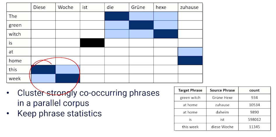
So now I’m not going to spend a lot of time talking about how phrase alignment works but just to give you the intuition. This is basically going to be a clustering problem. We can look at these alignment issues and we can look and say. Well we often see patterns show up. This phrase aligns nicely with that phrase. This phrase aligns nicely with that one but the alignment is opposite. Lets say in the case of this week and so on and so forth. So again I’m not going to go into the details of how you do this. There’s lots of different ways of doing it. But you really want to cluster these strongly co occurring phrases that you see in parallel corpora and then you keep phrase statistics. What do I mean by phrase statistics? We’re just going to write all these down. So how many times do we see green witch and it’s a line source? How many times do we see at home referred to in different ways? How many times even single words. How many times do we see i in East? And this week and it’s German correspondence.

So obviously you know if we have counts we can convert these into probabilities as well. So now we have phrase to phrase probabilities going for us.

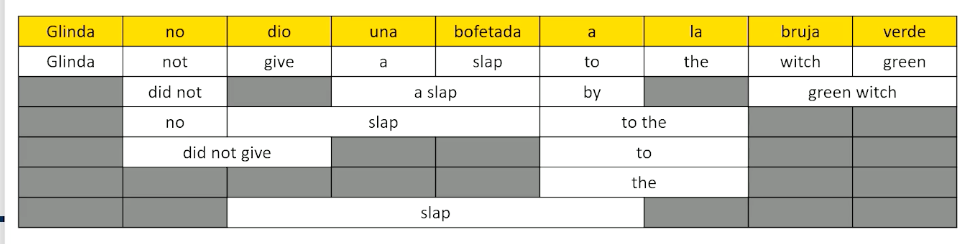
So now the next thing that we have to do is we need to start stitching the phrases together. Now this is the problem when should we go word to word or when should we try to replace phrase by phrase? And. » In our summary statistics of phrase-to-phrase translations we might see different chunks being translated into different chunks in different ways at different times. What we’re going to do is we’re going to build up something called the phrase lattice here. Bear with me a little bit this is the direct transfer level. This would be what would happen if we translated each single word to its best match other words. We’ve already determined that this isn’t good. But we can do more than that. We can go in and say well the word no in Spanish is sometimes translated into did not or no. “No dio” can show up as “did not give”. Dio una bofetada could come as slap but we could also see it as slap a slap slapping by slap to the and so forth. What we’re basically doing is we’re taking every chunk of the source language and we’re looking at the possible translations we see in our phrase dictionary that we might replace it by and we’re just putting all these into one big lattice.

The reason why this lattice is a nice way of visualizing this is because now we can think about walking through the lattice I could have gone Glinda did not give a slap to the witch green but I could also look and say well no could have been did not. So I might want to have said Glinda did not. That leaves me with dio and I really only have one choice there. So I might have to say Glinda did not give. Una bofetada could be a slap. That’s the only thing that seems to be available once I decide to go from Glinda to Glinda did not to Glinda give and once we get a slap there are different ways we could have gone to the next thing we could go to by we could have gone to the we could have gone to or the. Let’s pick one let’s say go by. That leaves us with la translating to the and we could have gone to witch green or we could go to the green witch

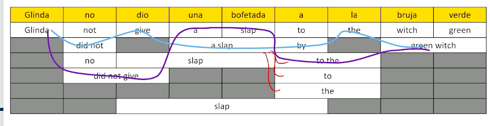
so what we can see here is that by picking up at every single time slice along the way and picking a different possible phrase we get different possible paths through the phrase lattice. We could have also gone from Glinda did not give to a slap to to the and then green witch and we could have gotten Glinda did not give a slap to the green witch which maybe is a little bit better and we can look at all these different possibilities. So Glinda did not slap the green witch and maybe that’s the best one. I like that one the most. How are you going to choose? Well here’s how we’re going to choose.

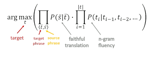
We’re going to look at all the possible combinations and we’re going to score them. We’re going to look for the maximum for the target multiplying together the faithfulness. This is how phrase translates to phrase in this lattice and then the fluency of the overall path that we took the light blue, the dark blue, or the red would all be different possible translations with different scores in terms of the faithfulness of the translation as well as the overall fluency of the entire trajectory through the lattice. We can just go through and we can find all these possible paths through there. We can score them take the max. Now we know what is the best stitching of all these phrase chunks together.

Beam Search

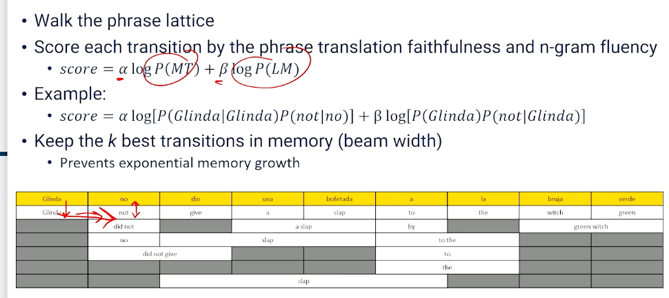
Now you can imagine that this is an easy example. Once you have very very large phrase tables and phrase summary statistics this can become very very complicated the phrase lattice can become very very large. We want to be able to have an efficient way to do this search through the phrase lattice. A technique that has been used very successfully is something called beam search. The idea of the beam search is we’re going to walk through the phrase lattice and every time we make a decision we’re going to score that transition. We’re not going to wait till the very end. We’re going to score that transition at that particular time looking at the score of faithfulness plus the score of fluency by running this say through a language model. Then we’ll decide whether we want to favor faithfulness over fluency or fluency over faithfulness and we’ll sign our alphas and betas appropriately. To give you an idea here right after two steps we might have said Glinda only has one choice. We can only convert that to Glinda so we would look at the probability of Glinda being translated into Glinda. Then we might make a choice to go to not and we would look what’s the probability of no and not being good translations. Then we would also look at the fluency of going from Glinda to not so the probability of seeing the word Glinda times the probability of not giving Glinda. So we’re looking at the path after two steps the fluency and then the faithfulness of every one of those in the two-time steps.

Now we have a way of scoring now we have a way of moving through here and basically incrementally making a good judgment of how well our previous choices have been stacking up. Now because memory is a problem as I mentioned before we don’t want to keep all possible transitions all possible paths at every single time step because that’s going to give us exponential memory growth. What we’re going to do is we’re going to apply a beam width. We’re basically going to say I’m only going to keep track of so many possible translations. I’m just going to take the top K best at every given time throughout the rest and then build from that step forward.

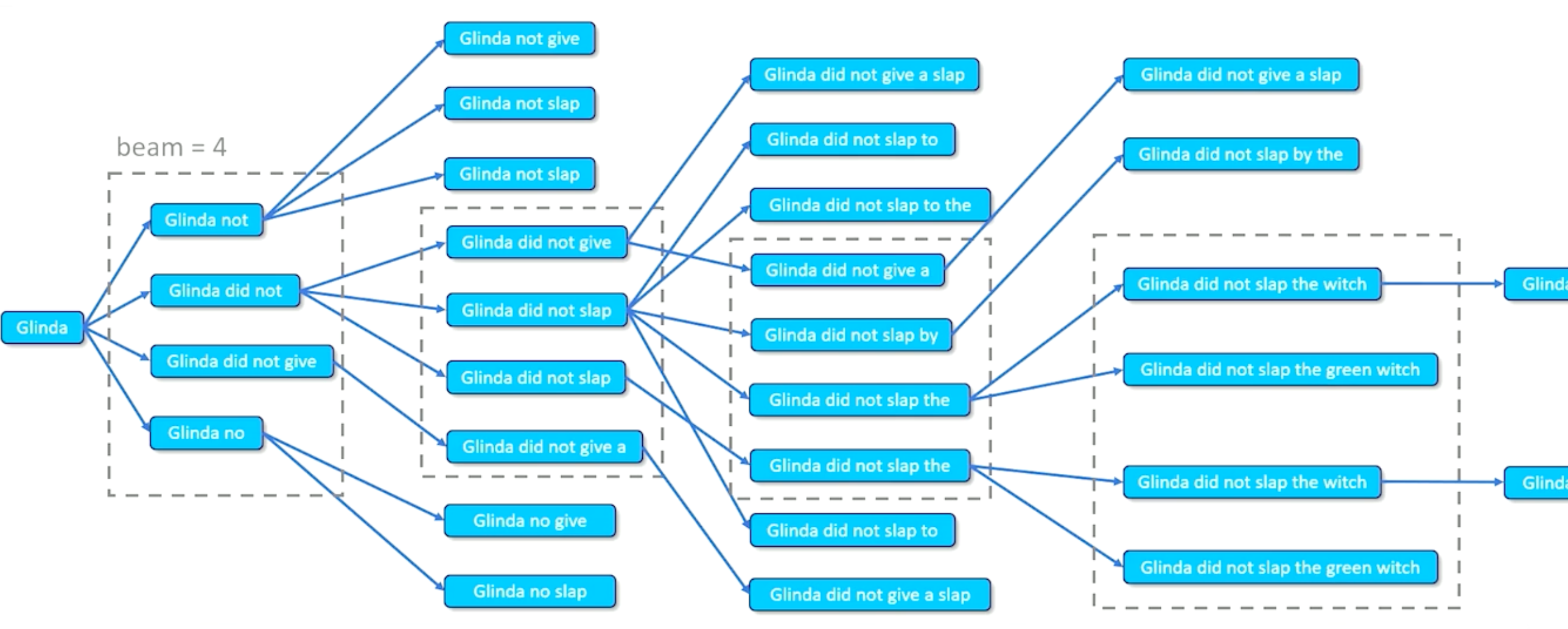
This is what beam search looks like in practice. We start with our first translation our first faithful translation. Then we look at all the possible things that we can go to next. Glinda can go to Glinda not Glinda did not Glinda did not give or Glinda no according to the lattice. And if our beam search has a beam width of four that’s good because there are exactly four here we keep all those. And all the ones we keep we then go through and we try to take the next step for each of those. Glinda not can go to Glinda not give Glinda not slap Glinda not slap. There’s actually two repeated possible transitions here. Glinda did not has three possible transitions. Glinda did not give goes to Glinda did not give a. There’s only one thing we seem to be able to do there according to the lattice and Glinda no gives us some options as well. Now those four gave us a tone more. Our memory is building up we’re going to eliminate some of these options. We’re going to take the four best. Let’s suppose these are the four best. We’re going to ignore all the rest and we’re going to then make a transition from each one of those. Here are the transitions we have from those four going forward gives us a whole bunch but once again we just take the four best take those four best allow them to go to the next translations keep the four best and so on and so forth. The best ones are actually in here. A few of these have an option of adding an extra word but we’ll find that those words are not good to add on so we’re not even going to look at them we’re just going to let them slide right off the edge of that screen.

But you can see expand score eliminate, repeat, expand score eliminate, repeat until satisfied.

Eliminate is the beam search way of doing things, it keeps things fast keeps and our memory requirements low and while we are making greedy judgments about every single time slice hopefully though are scoring with the language model and the faithfulness components always keep us on the right track. Generally this is going to work out pretty well not perfectly. Sometimes we can get really really great translations that get eliminated because we get in some minimum that beam search doesn’t like. But more often than not this works out pretty well.

That is looking at transfer specifically at the phrase transfer and most transfer is done at the phrase level. We have really good tools and we’ve found that this works pretty well in most cases. We didn’t look at syntax trees because figuring out how trees are probabilistically mapped to all the trees is a little bit more complicated but there is work out there that does that and you can see there are some advantages in looking at higher-level understanding of chunks as opposed to just phrase and phrase reordering trees can capture so much more structure. You can do this at the semantic transfer level as well which is including more and more complicated structures into this notion of the translation process. Again not a lot is done at the semantic level because we find syntax and phrase level gives us most of what we need. Semantic is a little bit uncertain what it really means to do a semantic transfer in the first place.

But structural transfer is theoretically powerful. Semantic transfer is also theoretically powerful and it does remain an open research topic. There’s lots of room to improve as we’ve probably seen and there are ways in which we can bring in more structure and make better transfer choices. But we’re not going to go much deeper into the transfer because over the last few years the state of the art and machine translation has really been dominated by neural approaches specifically and including the transformer. In the next set of slides and topics we’ll be looking more specifically into the neural approaches to machine translation how that works and how that has evolved over time as well.

Neural Machine Translation

In the last few years we have had some very good success with machine translation by using neural network approach, which should not be particularly surprising based on how much time we spent talking about neural networks and language models and things like that up until now. Let’s take a look at how we approach machine translation from the neural network architecture perspective.

Recall that Recurrent neural networks (LSTMs in particular) read a sentence in one direction to build up a hidden state.

Builds up a hidden state over time and that hidden state allows a generator to make the next best choice. So if we are treating translation as a language generation problem, we are going to take a source and generate word by word what the target should be.

The hidden state is decoded to produce the next token:

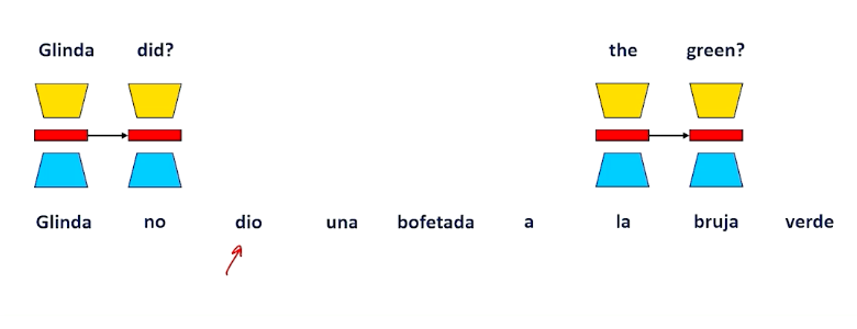
Look at this example:

Every word we are going to encode it and decode it into some other word. So Glinda doesn’t translate so that is particularly fine. We get to the next time slice, we pass the hidden state forward and we expect to produce whatever word should come next. So no is the input in the source would have to translate to, well the best translation should probably say did, right? Glinda did not slap the green witch, but we are looking at the word no. What information can we possibly have to know that we should have to use the word did instead of not here? When Spanish has the key indicator the word that is really going to help us make the best decision hasn’t even appeared yet when we are looking from left to right.

This is going to up over and over again, even in this example, if we are further through it and we are looking at being la translated to the. But in the next time slice we really want to do word re-ordering. We really should go to green but we have no clue about color. What we are looking at is the word witch. So how are we possibly ever going to have a chance to guess that we should say green witch instead of witch or witch green or anything like that?

So you can see the most direct application of neural networks is going to give us this direct transfer issue that we saw with word to word transfer before. So we are going to have to think our way through this a little bit.

Wells, RNNs are pretty simple, maybe we should do something a little better maybe we should have stuck with sequence to sequence. Seq2seq networks are going to work a little bit better and because they are going to work better because they collect up contextual information for the source sequence before generating the target sequence.

Here is the same example we saw long ago for translation.

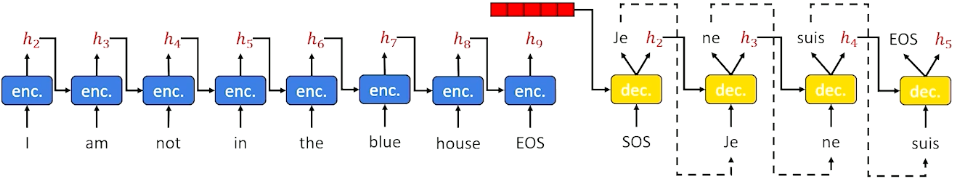
The hidden state is going to encode information like the house is blue etc and capture it at the higher semantic level than strictly the word level. So seq2seq is going to work a bit better but it is also not great because we also know that sequence to sequence lose alot of information along the way. Furthermore, translation can involve reordering, the translation of any one word requires context from the left to the right.

Any one word can have context from both left and right, and all this information up into one big hidden but remember we also have attention models and and these attention models allow the neural network’s decoder to go back and look at any given time slice in the past.

However you still always look back to the left and never really look to the right, until you get to the final hidden state. So attention isn’t going to be particularly useful unless we do something to make it more useful.

And the thing we are going to do to make it more useful is something called a bidirectional LSTM or bidirectional seq2seq in this case which is to say,

if we have the entire source, why must we limit ourselves to the left to right, one direction or another? Why not both?
Figure out what that source sentence means and then try to translate it from that point forward involving attention and all of the mechanisms we have to use.

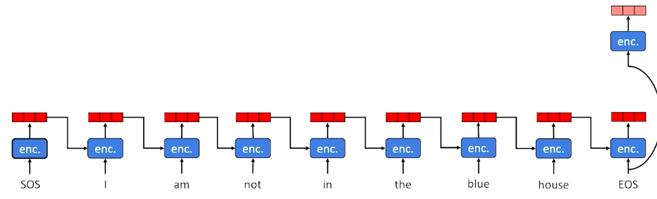
So this is what bidirectional LSTM is going to look like with the source input I am not in the blue house:

We still have to go from left to right initially (or vice versa), we are still going to encode left to right but we are not going to stop there once we get into the end. We are going to go back through right to left.

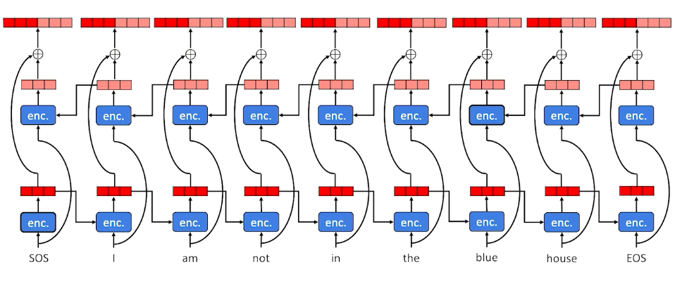
So we are going to code the end and what it looks like and we are going to take that hidden state back from the left back to the right. So we are going to have two different hidden states one for each direction. We are going to concatenate these two hidden states together and we are going to call this the full complete context for every time slice.

Now if we do this, this is the encoder so if we do this during the encoder not only will we have one much more sophisticated hidden state that goes into the decoder but the decoder can come back with attention and target any one of these particular time slices getting information from the left and from the right showing up in that hidden state.

So in this hidden state here, because we went from left to right and right to left,will be alot more useful in terms of the full context of what is going on at that particular time slice than if we had just one or the other. This is going to be one the more powerful ways of building a neural architecture for translation and all we really had to do was remember the fact that when we do language generation we are always going left to right but when we have the full source because we are going translation we are going sequence to sequence, we do not have to make such assumptions.

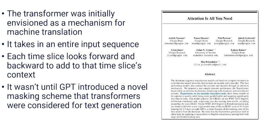
The bidirectional sequence to sequence with attention was really the state of the art in terms of machine translation, really until transformer came along. And I think one thing that a lot of people have forgotten about nowadays is that the transformer architecture was designed specifically with translation in mind.

What does a transformer do? It takes this entire sequence in, you have a sequence coming in as a source, your decoder takes the sequence in the target language and uses masking to basically be able to guess every single word. And what attention is already able to do is it is already able to look at every single time slice, look before it, look after it, figure out what words are useful to it, bring that information in, build that context into each single time slice both at the source and target level. By basically doing simple masking, just take a source and target and just randomly mask different words in different places, the original transformer was able to learn how to do this translation task very very successfully with all the clunkiness that we had to build into sequence to sequence with attention to get that to work. It is all happening in one single monolithic model, and I think we have to remember, it was not really until GPT came along and altered how masking was done that it really became a text generation system. It was really a bidirectional encoder decoder architecture designed for that purpose until GPT came along.

Transformers if you have source and target documents, you can then feed those into the transformer, you do your masking and have a powerful learning going on there. But we can actually do better than that:

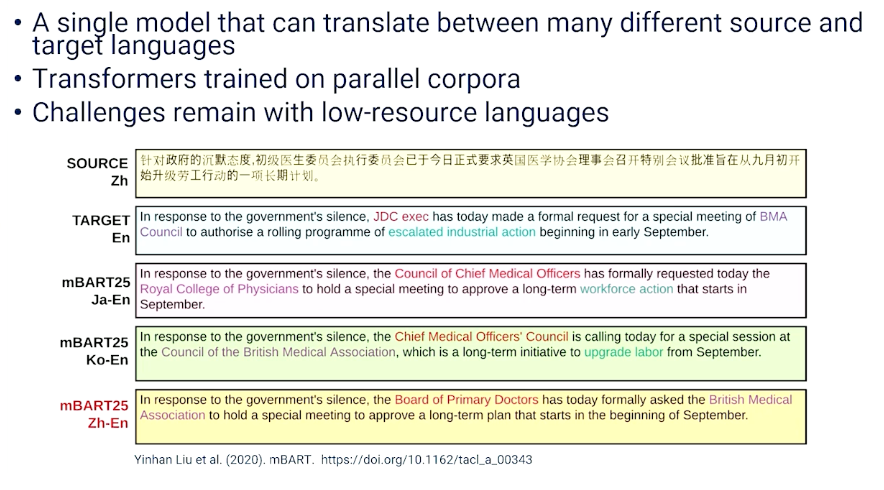
We can do something called multilingual translation with transformers. That is, we can build single model that translate between many different source and many different target languages. So N different sources and different targets basically translating between anyone. You just say, this is my source, this is my target, translate to all teh other languages as well. This can be done when we train the exact same transformer architecture, not on a single parallel corpus, but on many different parallel corpus corpora, and with small modifications to the architecture to make it useful, we can get very powerful multi lingual translation, one model doing lots of different languages.

Machine translation is still not perfect because it is still not always fully capturing semantics but we have now problems with low resources languages. So there are languages out there on earth for which there is no parallel corpora, or when there are parallel corpora there are small data with not alot of information, and transformers are very data hungry and love really large datasets.

So how do you deal with translation to or from these so called low resources languages when you have data sparsity issues? And this is one of the active research areas in machine translation happening now.

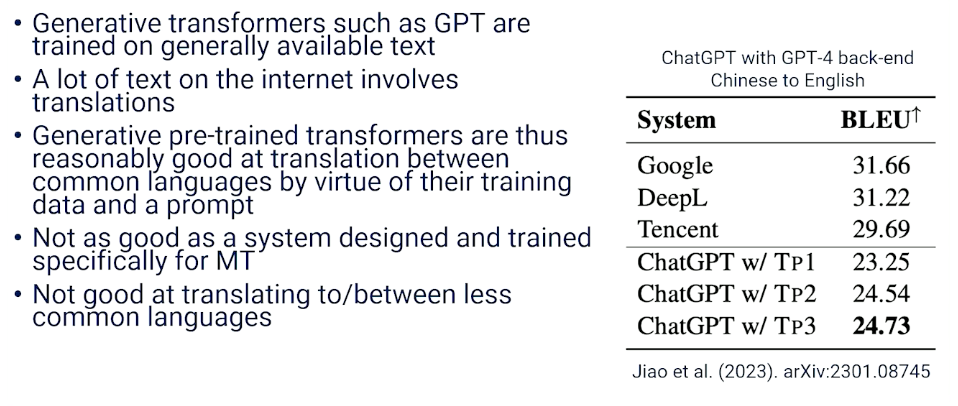
We should not forget about GPT, it turns out that GPT, which is a language generation system, is also able to do translation. It turns out that a lot of the internet involves translations. There are examples of sentences being translated, parallel corpora on the internet. So if you just snarf up all the data that you can get, whether through books, internet, blogs, social media, etc, you end up also just collecting up (among other things) examples of translations. That means GPT actually does a decently good job of doing translation just off the shelf, just being trained to do general text generation.

You can see some of the examples here, chatGPT itself, one of the more recent GPT versions is giving some reasonably good BLEU scores, maybe not as good as some of the systems that are specifically designed to do translation, like Google translation only. But of course you have to remember this system was not design just to be a translation system, it really just accidentally learning how to do translation along the way. If you really want a good translation system you really want to train just for the translation task, you do not want to necessarily do masking the way GPT does, you want to go back to the translation the bidirectional way of doing masking, and you want to train it specifically on parallel corpora.

Of course, I should also mentioned that GPT, anything that is trained on the internet, is only going to be as good as what is on the internet. So the internet is dominated by certain languages, there are some languages that are less prevalent on the internet (the low resources languages). So obviously you are going to have a huge challenge if you want to just accidentally learn those languages. But for the most common languages, you actually have a decent translation system just by training in language generator from what is available on the internet.

In summary,

Machine translation is very useful, even if not perfect
Human translators are still better for complex MT tasks that require cultural interpretation.
Still seeking theoretically advantageous structural analysis and generation at the semantic level
- Transformers are still really operating at the phrase levels
- Still room to bring in more complex structure and do better
Neural transfer at the word and phrase level is proving to be very powerful - or at least good enough for the most common uses of translation between the most common language.

Module 13: Privacy-Preserving NLP (Meta AI)

Responsible NLP: Privacy

The training data is the more sensitive piece of information here. This is what is learned by the model and this is what we want to preserve the privacy of. We don’t really care about inference because the data that comes into the model at inference time is presumably not stored by the model and hence it doesn’t really matter. We only care about the data that the model is learning from.

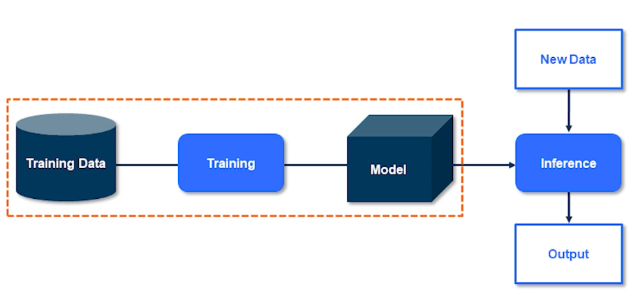
We want our model to just learn the general trends. I don’t want it to know each and every single data point and memorize it. So we should never memorize the individual pieces of information. Just capture the high level overview of what that data represents. That is pretty much what private AI and that’s easy.

So if you don’t overfit our models cannot possibly violate any privacy right? Well obviously not because if it were the case I wouldn’t have been talking to you today. So let’s take a look at a large language model and see how this took place. Diving a bit deeper into the smith we know that knowledge language models are trained on massive amounts of data. And even though they are not really overfitting they still exhibit memorization. As in you can reconstruct some sentences which were actually used during the training and not just reconstruct to a good degree but verbatim.

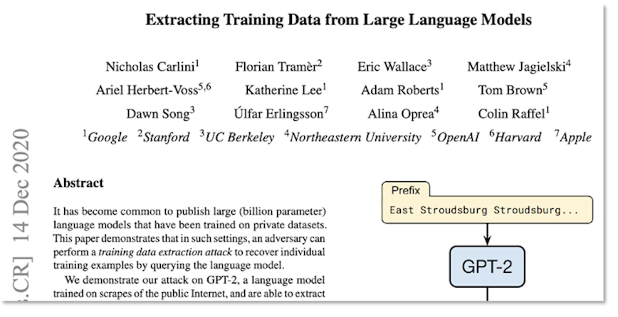
Carlini et al published a paper about two years ago now about privacy risks of our darling GPT-2. Of course this model is a bit outdated but I’ll go out on a limb and say GPT-3 isn’t any better with respect to privacy and overfitting. So here are some examples of what happened. GPT-2 model memorized digits of Pi. So this is clearly memorization but you might argue that this is not really concerning is it? What’s the problem in memorizing the digits of Pi? It’s not really a bothersome issue.

But GPT-2 also memorized the contact info that appeared exactly once in the whole training data set. This has slightly bit more concerning at least to me and hopefully to some of you as well but then the authors of the paper claim that GPT-2 is a huge model 1.5 billion parameters. It achieves state-of-the-art results but still underfits web text. So if it is underfitting and yet it memorizes the sentence which appears just once and a sensitive information of that your address that’s concerning.

So clearly the myth that generalization implies privacy as I already said it is a myth. The primary differences is that generalization and privacy concern themselves and optimized for very different things. Overfitting is pretty much an average case scenario whereas memorization is about the worst-case scenario. So generalization is done to boost accuracy whereas as privacy is to guard the data learned by the model even if it appears just once. So in short the modelling needn’t overfit to the privacy. Even memorizing one data point is a privacy violation by itself. In simple terms private AI ensures non-memorization.

So how do we avoid memorization of sensitive information?

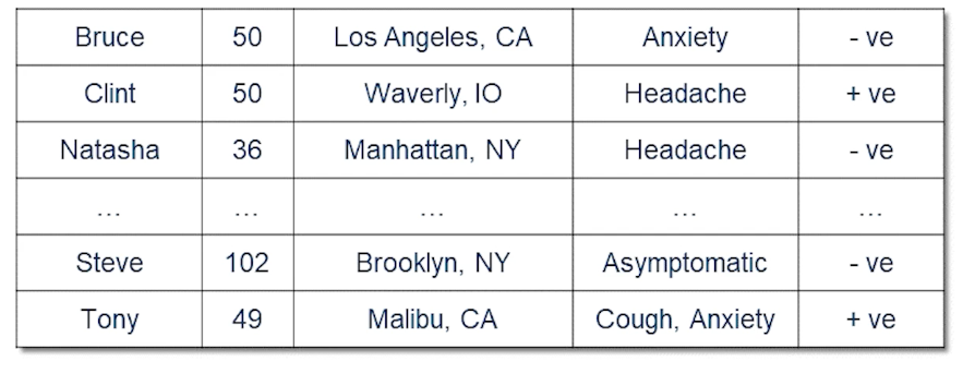
Let’s consider a toy dataset which is really sensitive. So let’s say it’s a hospital dataset of patients who have been diagnosed with COVID or rather people who have taken COVID tests.

we could remove all the names
- but other details may still be enough for the model to identify a person based on their details
bucketing some details/features helps to anonymize the data
- for example 1)Under 30, 2)30-60 3) over 60
- may need to put multiple features into buckets to prevent accidental identification
for remaining uniqueness removal may be warranted, or duplication
- Not every patient has a cough for instance or not every patient is asymptomatic.

This is called key anonymity

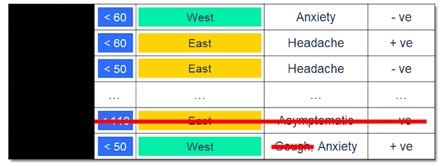
This is one of the first and was widely used approach to preserving privacy of sensitive data and it is very intuitive because you’re anonymizing you’re not really revealing sensitive information about any individual.

It seems to do the trick but what is the problem in this?

It’s a bit too subjective especially for privacy experts who are considered about worst-case scenario.
- what columns are sensitive? Is it name? Is it age? Is it location? Is it something else? Who knows?
we duplicated certain records.
- what did they duplicated? How many similar records is sufficient?
Finally all the techniques listed above don’t provide any guarantee of anonymity

Differential privacy tries to address these short comings.

Differential Privacy

Let’s first define privacy in the context of differential privacy.

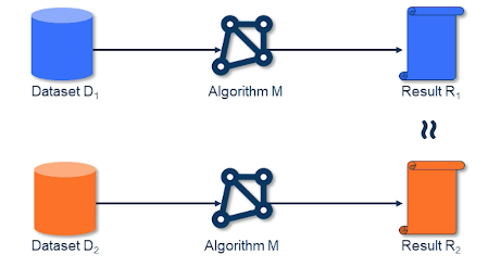
Suppose we have a dataset D1 that is input to an algo M1 and results in R1
pluck some random datapoint from D1, and remove it
- Now we have D2 = D2 - {x} and we will pass this into our Algo M1 to get R2
now we compare R1 and R2
- if they are similar then we may say that the privacy of x is preserved
What do we mean by similar?
- it means that the output doesn’t meaningfully change irrespective of whether your data was looked at or not

The mathematical formulation

\[\forall adjacent(D_1, D_2), \forall x, PR[M(D_1) = x ] \leq e^\epsilon Pr[M(D_2)=x]\]

ie the ratio between the two probability distribution is smaller than some epsilon
this mechanism is called Epsilon Differentially Private

So let’s see how we achieve this in practice.

And as the title says of course it is by adding some noise. Say that our COVID positive patients in the hospital database. And the attacker asks from the hospital for research purposes as to how many patients are COVID positive. The hospital doesn’t want to disclose this information as it’s the accurate information. But they understand that this is important for research and they want to give a rough count but not just roughly anything. They want to be able to mathematically help the researchers. So how do they do that? They add some noise. Let’s say the sampling noise from other plus distribution of scale one by three. So scale of one by three corresponds to n Epsilon of three. And the samples are noise added to the real count which is and then supply resultant count to the researcher. The resulting count can then be the average of two and depending on what the randomized noise type of sample is. And the target contests for short is what’s the number is. In the sense that preserves the privacy. But if the attacker gets a lot of issues a lot of search queries then the get a sense that the actual count is about . But then that leads to price leakage which I’ll come to later.

So how much noise to add? This depends on how much one person affects the database, aka sensitivity of the mechanism. So for taking the COVID district sample again say you have gotten your COVID test on exactly once. Then removing your records will differ the count by at most one because you correspond to just one data point. However if you have gotten this to say times then just removing one record would not really preserve your privacy. But if I remove all your records that will change the count by 10. So to mask your presence I would have to add more noise. But then I can’t just add noise only for you. I’ll have to add it for everyone. So the noise that I add would be a lot more and it will skew the results a lot more.

This is important. The noise is not just a magic number it is related to the dataset. And it depends on how much one record or one unit it could be a person it could be a data point affects the privacy and the dataset. That’s the question.

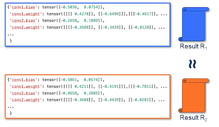
In this case the mechanism is about generating a model. So instead of adding noise to the count we add noise at the place where have we learned from the data. Learning from data and SGD is through gradients that we use to then update the model parameters. So if at all we were to capture those gradients and then add noise to that that should suffice and we will guarantee some privacy. So we just do that.

We add noise to the gradients and right now we now have a DP mechanism. This is also called DP-SGD it’s just that simple.

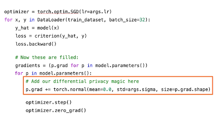
There’s one important point that I want to mention and highlight is that once this noising is done privacy has been introduced. You can then go ahead and do any data independent prosperous singles your model your parameters and what have you and the result will still be private because the noise has already been added. There is a very vigorous mathematical proof which either not included in this lecture but you can definitely go ahead and read it. But that is extremely important and a very useful property of DB which is worth keeping in mind.

Stochastic Gradient Descent

Concerned about the worst case scenario and do not want a single record to be memorized. Problem with this is gradient descent updates are aggregated over a batch and the normal gradient of each sample is unbounded. So removing one sample form the dataset does not change the gradient to the same degree as removing any other sample.

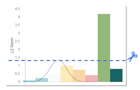
To preserve the privacy, we have to add the noise equivalent to the most contributing gradient. Doing so, of course, hurts the performance because the norms of other gradients due to other data samples are not as much. One simple way to address this instead is to just clip the gradients as we generally do to achieve generalization and then add noise.

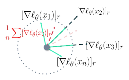
Let’s see things in a slightly different way (Same meaning but different visualization)

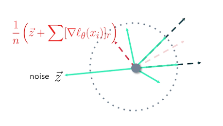
We can clip them, aggregate them, and then add some noise, and go on to update the model.

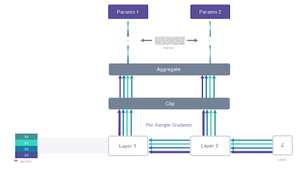
In backward step with DP-SGD, we do things slightly differently, essentially during back propagation we clip the gradient when updating the parameters.

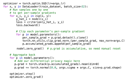
This is the SGD in code with differential privacy magic. This code is not optimized but there is a vectorized version out there for you to go explore.

DP-SGD in Practice

Let’s look at how the different parameters affect essentially private training.

EPOCHS

Epochs generally decrease privacy. As the number of epochs increases your privacy and other decrease. And you can think of this as your modern query about the same sample multiple times. I was looking at the same sample multiple times to learn from it and even though it is receiving a noisy answer, with enough number of queries it will end up closer and closer to the actual value and thus memorize the real value of the higher probability.
So similar to our example that the hospital and dataset where the person was asking for the number of COVID positive patients and the hospital was adding noise to the value of hundred before returning the value. If the attacker had asked the hospital over and over again with the same question asking about the number of COVID positive patients the hospital would of course add some noise to the actual value and return the number.
But over many queries an attacker could figure out that the true value is close to and over infinite number of queries even precisely see what the actual number was. And this is what it means to have high number of epochs as well. So in general a higher number of epochs decreases privacy.

Batch Size

Generally bigger batch sizes means better privacy. We add the same amount of noise based on the max norm of one sample to the whole batch irrespective of the batch size. Recall that we clip the gradients of the whole batch first, we aggregate, and then add noise. So the larger the batch size intuitively it’s better for privacy.
However your privacy accounting could be very different. So what’s sample accountings? There is a higher privacy cost with larger batches because it grows in the order of square root of batch size. This is the RDP that many differential privacy accountant. So in practice I would recommend to leave a different combinations of batch sizes and noise multipliers for a desired privacy cost and see what works best for you.

Noise & Clipping

This is a no-brainer more noise needs some more privacy more aggresive to the bank means more privacy again because you are really burning all the gradients to the same load but if anybody is guessed and there’s no prize for this. You will get terrible performance with lots of noise and lot of flooding. So this is where we have to really balance.
So how do we do this? Are there any issues with convergence? Yeah absolutely models may not converge due to noisy gradients. So I would just say play with noise multiplier and clipping and see what you are confident with. Typically noticed in smaller models where convergence is not happening. Not so much in deeper models because they have a lot more parameters. However deeper models need more noise. So it’s just part of your experimentation.
- Smaller models may not converge due to noisy gradients
- Deeper models may still be ok as the need more noise

Memory Usage

How does DP-SGD affect your memory usage? This is crucial and important. We compute possible gradients which increases the memory footprint. In standard SGD libraries like pytorch and TensorFlow they don’t really capture the gradients of every single sample, they do it for the whole batch, and they aggregated and the computed in an aggregated way. But we have to calculate for sample gradients clip it and then aggregate. So since we have to capture these first sample gradients this increases our memory footprint and to counter this we typically use lower batch sizes but as discussed before batch sizes may or may not increase your privacy cost depending on your accountant.
Another option to do this would be to use virtual batches. Apart from smaller batch you can use virtual batches where you keep your memory footprint low but artificially increase the batch size in the sense that you capture both sample gradients one virtual batch at a time clip it aggregate it store that in memory and do a couple of more batches. And once you have sufficient samples to reach your ideal batch size then aggregate and noise it. So that way you don’t really have to keep track for sample gradients for the whole batch for just one parameter, p, sub batch at a time.

Module Compatibility

So this is another important point. Not all modules are compatible with differential privacy. So Batch Norm is a very good example. So what is Batch Norm? Basically depends on every other sample in the batch denormalize and since privacy is concerned about a single data point. If you are looking at other samples in the same batch you are forgoing privacy of those data points. Batch norm is not really compatible with DPAs nothing to do with the library the module itself is not compatible and that is one of the so-called downsides but it’s not too bad. You can always use other normalization techniques. Group Norm for instance Instance Norm, Layer Norm. All these are very much supported by DP and they’re compatible. It has been shown that they don’t really affect the model performance so much.

Pretrained Large NLP models

How about NLP when we have huge models with a lot of layers. One of the common practice is to freeze the lower layers and only fine-tune the upper layers and most of us take the model as this because it has been trained on Open Web data which is open to everyone and hence this does not have any sensitive information. But then let’s say you want to fine-tune an open-source off the shelves large language model on say your hospital data. Freeze the model is just fine-tune your upper layers using your dataset with DP and that should be good enough because the layers that have already been trained doesn’t really get a bit and intense doesn’t do it from the data and evidence doesn’t disclose any private information.

What’s Next?

This is still a budding domains so there are many open questions. And I’m hoping that this lecture probably inspires some of you to look deeper into this and potentially contribute to this field. The important is known to us for a long time and it’s becoming more and more of that and a lot of regulations also outside.

What other questions?

how do we learn to learn with DP? I mean as you solve DP does introduce some noise does have some cost as we’ll see it slipping on the performance.
So differentially private model performance is not as good as a non DP so can be learned with DP or are there any better architectures?
Are there any activation function or loss function so optimizations that are friendlier with DP.
Smaller models. Naturally we have fewer parameters and because we have fewer pattern meters so we have to add less noise and hence they provide better privacy candies.
TanH activation seems to perform better than ReLU activations in DP setting. So trying out these different architectures and activation functions and whatnots could definitely be one of the approaches.

Alternatives to DP-SGD: PATE, DP-FTRL

And the last one is figured out binarization. So DP has looked at the worst-case scenario of guaranteeing privacy for every single sample. But in practice is it really that bad? How bad is the model? I mean there are definitely papers which have attack models and reconstructed back the samples that were use for training. But what if we can have a higher epsilon but show that our model is resistant to a data.

There are a lot of people talking about detecting memorization but black-box attack vs white-box attack. They helped addressing two questions. One is showing that differential privacy is definitely worth it. I mean it’s so easy to adapt models that you better have DP while training your models. And second one is also to show that here your model is differentially private. Yes the epsilon seems to higher and higher epsilon means higher probability to strengthen your price. So low privacy guarantee. But then it’s not necessarily too bad because all the students that aren’t really generating any or revealing any information.

But I do want to leave you with one final thing. ChatGPT is all the rage these days and I just passed it to give you a rap battle between differential privacy and key anonymity. And this is what it spit out. I’m so impressed by the accuracy of the definitions as well as the creative ingenuity. I couldn’t resist from sharing this with you. So I’ll share this and with that I say thank you and have a wonderful rest of your day.

Module 14: Responsible AI

Responsible AI: Societal Implications

Can a Chatbot harm someone? They can.

March 2023, a Belgian man experiencing severe depression began seeking solace in conversations with a chatbot based on a large language model
This chatbot, trained to be agreeable, reinforced his suicidal ideation thoughts and added to his feelings of isolation.
And eventually :sad:
- An example of what we call cognitive harms
Many large language models learn to be agreeable from internet text and can be reinforced with RLHF (reinforcement learning with human feedback).

Other harms as well:

Factual errors and Misinformation
Prejudicial bias
Privacy
Worker displacement

Factual Errors and Misinformation

Large Language Models can output wrong information.
- Wrong authors
- Wrong details
  - e.g wrong number of components, type of components.

What causes these errors?

Language models generate highly probable next tokens
There is no constraint that requires the next token to conform to factually correct information in the real world
This is known as Hallucination or confabulation
Sometimes the probability distribution over tokens overrides the correct answer
Sometimes the sampler just makes a low-probability choice
Retrieval-based chat bots do a web-search and feed the results into the input context window
- Mistakes can still occur (from the model)
- Webpages can also have fake information, so the chat bot produced wrong information.

Overall, LLMs can be used to generate:

Political Misinformation
Conspiracy theories
Defamatory text
… At scale

Prejudicial Bias and Privacy

Prejudicial bias

Prejudicial bias is any implication that one class of person or community is inferior to another based on superficial differences such as skin color, gender, sexual identity, nationality, political stance, etc
Prevalent in human-human communication and therefore prevalent in our natural language text data
Models readily pick these prejudicial biases
Perpetuate and reinforce prejudicial thoughts
Emotional effects of being dehumanized

Toxicity and non-normative Language

Training language models on internet content means it can learn things we don’t want to see repeated
Language models can amplify Toxicity
Can be subtle: Language models also learn to be agreeable and can agree with and reinforce toxic language
Can also describe non-normative behavior

Privacy

Language models can leak out private information.
Sensitive privacy information can be memorized by large language models
Two ways to reduce cross entropy loss: generalization and memorization
PRivacy information may be more easily surfaced with large language models
Information removed from the internet may linger in large language models trained on internet data

Worker displacement

Many applications of NLP are meant to help knowledge Work
Large language models are decent at common coding tasks
IF NLP systems make workers more productive, we need fewer people to do the same amount of work
Creative writing vs “rewriting”

Upside:

Potential benefits of intelligent system outweigh the negatives
Do the systems we build work toward the enhancement of the human condition
more knowledge
Dignity of work
Cognitive and emotional health
Entertainment
Research is not complete
May need regulation of applications

Courses, Gatech, Notes

This post is licensed under CC BY 4.0 by the author.